Chapter 10
Using Significance Tests
IN THIS CHAPTER
 Understanding estimation statistics
Using the Student’s t-distribution test functions
Analyzing probabilities and results with the chi square functions
When you have data from a population, you can draw a sample and run your statistical analysis on the sample. You can also run the analysis on the population itself. Is the mean of the sample data the same as the mean of the whole population? You can calculate the mean of both the sample and the population and then know precisely how well the sample represents the population. Are the two means exact? Off a little bit? How much different?
The problem with this, though, is that getting the data of the entire population in the first place isn’t always feasible. On average, how many miles per gallon does a Toyota Camry get after 5 years on the road? You cannot answer this question to an exact degree, because it’s impossible to test every Camry out there.
Instead, you infer the answer. Testing a handful, or sample, of Camrys is certainly possible. Then the mean gas mileage of the sample is used to represent the mean gas mileage of all 5-year-old Camrys. The mean of the sample group will not necessarily match the mean of the population, but it is the best value that can be attained.
This type of statistical work is known as estimation, or inferential statistics. In this chapter, I show you the functions that work with the Student’s t-test, useful for gaining insight into the unknown population properties. This is the method of choice when you’re using a small sample — say, 30 data points or less.
The tests presented in this chapter deal with probabilities. If the result of a test — a t-test, for example — falls within a certain probability range, the result is said to be significant. Outside that range, the result is considered to be nonsignificant. A common rule of thumb is to consider probabilities less than 5 percent, or 0.05, to be significant, but exceptions to this rule exist.
 The Student’s t-test has nothing to do with students. The originator of the method was not allowed to use his real name due to his employer’s rules. Instead, he used the name Student.
Testing to the T
The TTEST function returns the probability that two samples come from populations that have the same mean. For example, a comparison of the salaries of accountants and professors in New York City is under way. Are the salaries, overall (on average), the same for these two groups? Each group is a separate population, but if the means are the same, the average salaries are the same.
Polling all the accountants and professors isn’t possible, so a sample of each is taken. Twenty-five random members of each group divulge their salaries in the interest of the comparison. Figure 10-1 shows the salaries of the two groups, as well as the results of the TTEST function.
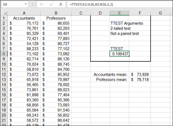
FIGURE 10-1: Comparing salaries.
The TTEST function returns 10.6 percent (0.106437) based on how the arguments of the function were entered. This percentage says there is a 10.6 percent probability that the mean of the underlying populations are the same. Said another way, this is the likelihood that the mean of all accountant salaries in New York City matches the mean of all professor salaries in New York City. The formula in cell E8 is =TTEST(A2:A26,B2:B26,2,2).
The arguments of the TTEST function are listed in Table 10-1.
TABLE 10-1 Arguments of the TTEST Function
Argument |
Comment |
Array 1 |
The reference to the range of the first array of data. |
Array 2 |
The reference to the range of the second array of data. |
Tails |
Either 1 or 2. For a one-tailed test, enter 1. For a two-tailed test, enter 2. |
Type |
Type of t-test to perform. The choice is 1, 2, or 3. A number 1 indicates a paired test. A number 2 indicates a two-sample test with equal variance. A number 3 indicates a two-sample test with unequal variance. |
The third argument of TTEST tells whether to conduct a one-tailed or two-tailed test. A one-tailed test is used when there is a question of whether one set of data is specifically larger or smaller than the other. A two-tailed test is used to tell whether the two sets are just different without specifying larger or smaller.
The first two arguments to TTEST are the ranges of the two sets of values. A pertinent consideration here is how the two sets of data are related. The sets could be comprised of elements that have a corresponding member in each set. For example, there could be a set of “before” data and a set of “after” data.
Seedling |
Height at Week 1 |
Height at Week 2 |
#1 |
4 inches |
5 inches |
#2 |
3¾ inches |
5 inches |
#3 |
4½ inches |
5½ inches |
#4 |
5 inches |
5 inches |
This type of data is entered in the function as paired. In other words, each data value in the first sample is linked to a data value in the second sample. In this case, the link is due to the fact that the data values are “before” and “after” measurements from the same seedlings. Data can be paired in other ways. In the salary survey, for example, each accountant may be paired with a professor of the same age to ensure that length of time on the job does not affect the results. In this case, you would also use a paired t-test.
When you're using TTEST for paired samples, the two ranges entered for the first and second arguments must be the same size. When you’re comparing two independent (unpaired) samples, the two samples don’t have to be the same size.
 Use TTEST to determine the probability that two samples come from the same population.
Here’s how to use the TTEST function:
- Enter two sets of data.
- Position the cursor in the cell where you want the result to appear.
- Type =TTEST( to start the function.
- Drag the pointer over the first list or enter the address of its range.
- Type a comma (,).
- Drag the pointer over the second list or enter the address of its range.
- Type a comma (,).
- Type 1 for a one-tailed test, or type 2 for a two-tailed test.
- Type a comma (,).
- Enter one of the following:
- 1 for a paired test
- 2 for a test of two samples with equal variance
- 3 for a test of two samples with unequal variance
- Type a ).
If you’ve ever taken a statistics course, you may recall that a t-test returns a t-value, which you then had to look up in a table to determine the associated probability. Excel’s TTEST function combines these two steps. It calculates the t-value internally and determines the probability. You never see the actual t-value, just the probability — which is what you’re interested in anyway!
The TDIST function returns the probability for a given t-value and degrees of freedom. You would use this function if you had a calculated t-value and wanted to determine the associated probability. Note that the TTEST function doesn’t return a t-value but a probability, so you wouldn’t use TDIST with the result that is returned by TTEST. Instead, you would use TDIST if you had one or more t-values calculated elsewhere and needed to determine the associated probabilities.
TDIST takes three arguments:
- The t-value
- The degrees of freedom
- The number of tails (one or two)
A t-distribution is similar to a normal distribution. The plotted shape is a bell curve. However, a t-distribution differs, particularly in the thickness of the tails. How much so is dependent on the degrees of freedom. The degrees of freedom roughly relate to the number of elements in the sample, less one. All t-distributions are symmetrical around 0, as is the normal distribution. In practice, however, you always work with the right half of the curve — positive t-values.
To use the TDIST function, follow these steps:
- Position the cursor in the cell where you want the result to appear.
- Type =TDIST( to start the function.
- Enter a value for t or click a cell that has the value.
- Type a comma (,).
- Enter the degrees of freedom.
- Type a comma (,).
- Enter one of the following:
- 1 for a one-tailed test
- 2 for a two-tailed test
- Type a ).
 If the t-value is based on a paired test, the degrees of freedom is equal to 1 less than the count of items in either sample. (Remember, the samples are the same size.) When the t-value is based on two independent samples, the degrees of freedom = (count of sample-1 items – 1) + (count of sample-2 items – 1).
The TINV function produces the inverse of TDIST. That is, TINV takes two arguments — the probability and the degrees of freedom — and returns the value of t. To use TINV, follow these steps:
- Position the cursor in the cell where you want the result to appear.
- Type =TINV( to start the function.
- Enter the probability value (or click a cell that has the value).
- Type a comma (,).
- Enter the degrees of freedom.
- Type a ).
Comparing Results with an Estimate
The chi square test is a statistical method for determining whether observed results are within an acceptable range compared with what the results were expected to be. In other words, the chi square is a test of how well a before set of results and an after set of results compare. Did the observed results come close enough to the expected results that you can safely assume that there is no real difference? Or were the observed and expected results far enough apart that you must conclude that there is a real difference?
A good example is flipping a coin 100 times. The expected outcome is 50 times heads, 50 times tails. Figure 10-2 shows how a chi square test statistic is calculated in a worksheet without any functions.
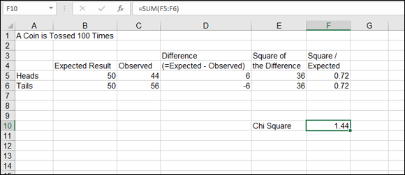
FIGURE 10-2: Calculating a chi square.
Cells B5:B6 show the expected results — that heads and tails each show up 50 times. Cells C5:C6 show the observed results. Heads appeared 44 times, and tails appeared 56 times. With this information, here is how the chi square test statistic is calculated:
- For each expected and observed pair, calculate the difference as (Expected – Observed).
- Calculate the square of each difference as (Expected – Observed)2.
- Divide the squares from Step 2 by their respective expected values.
- Sum the results of Step 3.
Of course, a comprehensive equation can be used for the first three steps, such as =(expected - observed)^2/expected.
The result in this example is 1.44. This number — the chi square value — is looked up in a table of chi square distribution values. This table is a matrix of degrees of freedom and confidence levels. Seeing where the calculated value is positioned in the table for the appropriate degrees of freedom (one less than the number of data points) shows you the probability that the difference between the expected and observed values is significant. That is, is the difference within a reasonable error of estimation, or is it real (for example, caused by an unbalanced coin)?
You can find the table of degrees of freedom and confidence levels in the appendix of a statistics book or on the Internet.
The CHISQ.TEST function returns the probability value (p) derived from the expected and observed ranges. The function has two arguments: the range of observed (or actual) values and the range of expected values. These ranges must, of course, contain the same number of values, and they must be matched (first item in the expected list is associated with the first item in the observed list, and so on). Internally, the function takes the degrees of freedom into account, calculates the chi square statistic value, and computes the probability.
Use the CHISQ.TEST function this way:
- Enter two ranges of values as expected and observed results.
- Position the cursor in the cell where you want the result to appear.
- Type =CHISQ.TEST( to start the function.
- Drag the cursor over the range of observed (actual) values or enter the address of the range.
- Type a comma (,).
- Drag the cursor over the range of expected values, or enter the address of the range.
- Type a ).
Figure 10-3 shows a data set of expected and actual values. The chi square test statistic is calculated as before, delivering a value of 1.594017, shown in cell F12. The CHISQ.TEST function, in cell D14, returns a value of 0.953006566 — the associated probability. CHISQ.TEST doesn’t return the chi square statistic but the associated probability.
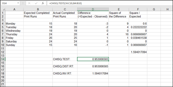
FIGURE 10-3: Determining probability.
Now tie in a relationship between the manually calculated chi square and the value returned with CHISQ.TEST. If you looked up your manually calculated chi square value (1.59) in a chi square table for degrees of freedom of 6 (one less than the number of observations), you would find it associated with a probability value of 0.95. Of course, the CHISQ.TEST function does this for you, returning the probability value, which is what you’re after. But suppose that you’ve manually calculated chi square values and want to know the associated probabilities. Do you have to use a table? Nope — the CHISQ.DIST.RT function comes to the rescue. Furthermore, if you have a probability and want to know the associated chi square value, you can use the CHISQ.INV.RT function.
The RT in the CHISQ.DIST.RT and CHISQ.INV.RT functions is the abbreviation for Right Tail. The functions in the configuration work with the right tail of the distribution.
Figure 10-3 earlier in this chapter demonstrates the CHISQ.DIST.RT and CHI.SQ.INV.RT functions as well. CHISQ.DIST.RT takes two arguments: a value to be evaluated for a distribution (the chi square value, 1.59 in the example) and the degrees of freedom (6 in the example). Cell D16 displays 0.953006566, which is the same probability value returned by the CHISQ.TEST function — just as it should be! The formula in cell D16 is =CHISQ.DIST.RT(F12,6).
CHISQ.TEST and CHISQ.DIST.RT both return the same probability value but calculate the result with different arguments. CHISQ.TEST uses the actual expected and observed values and internally calculates the test statistic to return the probability. This happens behind the scenes; just the probability is returned. CHISQ.DIST.RT needs the test statistic fed in as an argument.
To use the CHISQ.DIST.RT function, follow these steps:
- Position the cursor in the cell where you want the result to appear.
- Type =CHISQ.DIST.RT( to start the function.
- Click the cell that has the chi square test statistic.
- Type a comma (,).
- Enter the degrees of freedom.
- Type a ).
The CHISQ.INV.RT function rounds out the list of chi square functions in Excel. CHISQ.INV.RT is the inverse of CHISQ.DIST.RT. That is, with a given probability and degrees of freedom number, CHISQ.INV.RT returns the chi square test statistic.
Cell D18 in Figure 10-3 earlier in this chapter has the formula =CHISQ.INV.RT(D14,6). This returns the value of the chi square: 1.594017094. CHISQ.INV.RT is useful when you know the probability and degrees of freedom and need to determine the chi square test statistic value.
To use the CHISQ.INV.RT function, follow these steps:
- Position the cursor in the cell where you want the result to appear.
- Type =CHISQ.INV.RT( to start the function.
- Click the cell that has the probability.
- Type a comma (,).
- Enter the degrees of freedom.
- Type a ).
Working with inferential statistics is difficult! I suggest further reading to help with the functions and statistical examples discussed in this chapter. A great book is Statistics For Dummies, 2nd Edition, by Deborah J. Rumsey (John Wiley & Sons, Inc.).