Chapter 16

Writing Home About Text Functions

IN THIS CHAPTER

Assembling, altering, and formatting text

Figuring out the length of text

Comparing text

Searching for text

A rose is still a rose by any other name. Or maybe not, when you use Excel’s sophisticated text-manipulation functions to change it into something else. Case in point: You can use the REPLACE function to change a rose into a tulip or a daisy, literally!

Did you ever have to work on a list in which people’s full names are in one column, but you need to use only their last names? You could extract the last names to another column manually, but that strategy gets pretty tedious for more than a few names. What if the list contains hundreds of names? This is just one example of text manipulations that you can do easily and quickly with Excel’s text functions.

Breaking Apart Text

Excel has three functions that are used to extract part of a text value (often referred to as a string). The LEFT, RIGHT, and MID functions let you get to the parts of a text value that their name implies, extracting part of a text value from the left, the right, or the middle. Mastering these functions gives you the power to literally break text apart.

How about this? You have a list of codes of inventory items. The first three characters are the vendor ID, and the other characters are the part ID. You need just the vendor IDs. How do you do this? Or how do you get the part numbers not including the vendor IDs? Excel functions to the rescue!

Bearing to the LEFT

The LEFT function lets you grab a specified number of characters from the left side of a larger string. All you do is tell the function what or where the string is and how many characters you need to extract.

Figure 16-1 demonstrates how the LEFT function isolates the vendor ID in a hypothetical product code list (column A). The vendor ID is the first three characters in each product code. You want to extract the first three characters of each product code and put them in column B. You put the LEFT function in column B with the first argument, specifying where the larger string is (column A) and the second argument specifying how many characters to extract (three). See Figure 16-1 for an illustration of this worksheet with the LEFT formula visible in the Formula Bar. (What’s column C in this worksheet? I’ll get to that in the next section.)

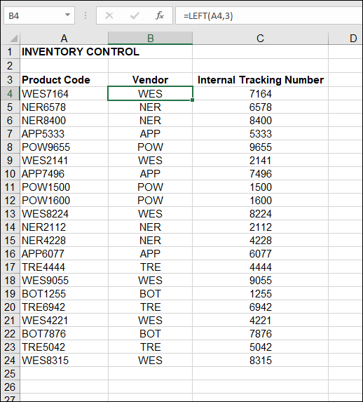
FIGURE 16-1: Getting the three left characters from a larger string.

What if you ask LEFT to return more characters than the entire original string contains? No problem. In this case, LEFT simply returns the entire original string. The same is true for the RIGHT function, explained in the next section.

The LEFT function is really handy and so easy to use. Try it yourself:

1. Position the cursor in the cell where you want the extracted string displayed.
2. Type =LEFT( to start the function.
3. Click the cell containing the original string or enter its address.
4. Type a comma (,).

5. Enter a number.

   This number tells the function how many characters to extract from the left of the larger string. If you enter a number that is equal to or larger than the number of characters in the string, the whole string is returned.

6. Type a ) and press Enter.

Swinging to the RIGHT

Excel does not favor sides. Because there is a LEFT function, there also is a RIGHT function. RIGHT extracts a specified number of characters from the right of a larger string. It works pretty much the same way as the LEFT function.

Column C in Figure 16-1 earlier in this chapter uses the RIGHT function to extract the rightmost four characters from the product codes. Cell C4, for example, has this formula: =RIGHT(A4,4).

Here's how to use the RIGHT function:

1. Position the cursor in the cell where you want the extracted string displayed.
2. Type =RIGHT( to start the function.
3. Click the cell containing the original string or enter its address.
4. Type a comma (,).

5. Enter a number.

   This number tells the function how many characters to extract from the right of the larger string. If you enter a number that is equal to or larger than the number of characters in the string, the whole string is returned.

6. Type a ) and press Enter.

Use LEFT and RIGHT to extract characters from the start or end of a text string. Use MID to extract characters from the middle.

Staying in the MIDdle

MID is a powerful text-extraction function. It lets you pull out a portion of a larger string — from anywhere within the larger string. The LEFT and RIGHT functions allow you to extract from the start or end of a string, but not the middle. MID gives you essentially complete flexibility.

MID takes three arguments: the larger string (or a reference to one), the character position to start at, and how many characters to extract. Here’s how to use MID:

1. Position the cursor in the cell where you want the extracted string displayed.
2. Type =MID( to start the function.
3. Click the cell that has the full text entry or enter its address.
4. Type a comma (,).

5. Enter a number to tell the function which character to start the extraction from.

   This number can be anything from 1 to the full count of characters of the string. Typically, the starting character position used with MID is greater than 1. Why? If you need to start at the first position, you may as well use the simpler LEFT function. If you enter a number for the starting character position that is greater than the length of the string, nothing is returned.

6. Type a comma (,).

7. Enter a number to tell the function how many characters to extract.

   If you enter a number that is greater than the remaining length of the string, the full remainder of the string is returned. For example, if you tell MID to extract characters 2 through 8 of a six-character string, MID returns characters 2 through 6.

8. Type a ) and press Enter.

Here are some examples of how MID works:

Example	Result
=MID("APPLE",4,2)	LE
=MID("APPLE",4,1)	L
=MID("APPLE",2,3)	PPL
=MID("APPLE",5,1)	E

Figure 16-2 shows how the MID function helps isolate the fourth and fifth characters in the hypothetical inventory shown in Figure 16-1. These characters could represent a storage-bin number for the inventory item. The MID function makes it easy to extract this piece of information from the larger product code.

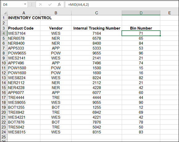
FIGURE 16-2: Using MID to pull characters from any position in a string.

Finding the long of it with LEN

The LEN function returns a string’s length. It takes a single argument: the string being evaluated. LEN is often used with other functions, such as LEFT or RIGHT.

Manipulating text sometimes requires a little math. For example, you may need to calculate how many characters to isolate with the RIGHT function. A common configuration of functions to do this is RIGHT, SEARCH, and LEN, like this:

=RIGHT(A1,LEN(A1)- SEARCH(" ",A1))

This calculates the number of characters to return as the full count of characters less the position where the space is. Used with the RIGHT function, this returns the characters to the right of the space.

The LEN function is often used with other functions, notably LEFT, RIGHT, and MID. In this manner, LEN helps determine the value of an argument to the other function.

Here’s how to use LEN:

1. Position the cursor in the cell where you want the results to appear.
2. Type =LEN( to begin the function.
3. Perform one of these steps:
   • Click a cell that contains text.
   • Enter the cell’s address.
   • Enter a string enclosed in double quotation marks.
4. Type a ) and press Enter.

Putting Text Together with CONCATENATE

The CONCATENATE function pulls multiple strings together into one larger string. A good use of this is when you have a column of first names and a column of last names and need to put the two together to use as full names.

CONCATENATE takes up to 255 arguments. Each argument is a string or a cell reference, and the arguments are separated by commas. The function does not insert anything, such as a space, between the strings. If you need to separate the substrings, as you would with the first name and last name example, you must explicitly insert the separator. Figure 16-3 makes this clear. You can see that the second argument to the CONCATENATE function is a space.

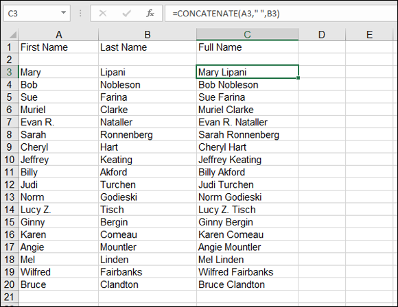
FIGURE 16-3: Putting strings together with CONCATENATE.

In Figure 16-3, the full names displayed in column C are concatenated from the first and last names in columns A and B, respectively. In the function’s arguments, enter a space between the references to cells in columns A and B. You enter a space by enclosing a space between double quotation marks, like this: " ".

There is another way to concatenate strings. You can use the ampersand (&) character instead and skip using CONCATENATE. Another way to create the full names shown in Figure 16-3 is to enter the following formula in the target cell: =A3 & " " & B3. Either method gets the job done. There really is no compelling reason to use one over the other; it's up to you, empowered user!

You can give this a whirl on your own. You probably have a list of names somewhere in an Excel workbook. Open that workbook, or at least enter first names and last names on your own, and then follow these steps:

1. Position the cursor in an empty column, in the same row as the first text entry, and type =CONCATENATE( to start the function.
2. Click the cell that has the first name, or enter its address.
3. Type a comma (,).

4. Enter a space inside double quotation marks.

   It should look like this: " ".

5. Type a comma (,).
6. Click the cell that has the last name or enter its address.
7. Type a ) and press Enter.
8. Use the fill handle to drag the function into the rows below, as many rows as there are text entries in the first column.

You can combine text strings in two ways: Use the CONCATENATE function or use the ampersand (&) operator.

Changing Text

There must be a whole lot of issues about text. I say that because a whole lot of functions let you work with text. There are functions that format text, replace text with other text, and clean text. (Yes, text needs a good scrubbing at times.) There are functions just for making lowercase letters into uppercase and uppercase letters into lowercase.

Making money

Formatting numbers as currency is a common need in Excel. The Format Cells dialog box or the Currency Style button in the Number Formatting options of the Home tab of the Ribbon are the usual places to go to format cells as currency. Excel also has the DOLLAR function. On the surface, DOLLAR seems to do the same thing as the similar currency formatting options but has some key differences:

• DOLLAR converts a number to text. Therefore, you cannot perform math on a DOLLAR value. For example, a series of DOLLAR amounts cannot be summed into a total.
• DOLLAR displays a value from another cell. As its first argument, DOLLAR takes a cell address or a number entered directly in the function. DOLLAR is handy when you want to preserve the original cell’s formatting. In other words, you may need to present a value as currency in one location but also let the number display in its original format in another location. DOLLAR lets you take the original number and present it as currency in another cell — the one you place the DOLLAR function in.
• DOLLAR includes a rounding feature. DOLLAR has a bit more muscle than the currency style. DOLLAR takes a second argument that specifies how many decimal places to display. When negative values are entered for the second argument, this serves to apply rounding to the digits on the left side of the decimal.

Figure 16-4 shows how the DOLLAR function can display various numeric values just the way you want. At the bottom of the worksheet is an area of detailed revenues. At the top is a summary that uses DOLLAR.

FIGURE 16-4: Using DOLLAR to round numbers and format them as currency.

Unless a cell has been formatted otherwise, you can tell the type of entry by alignment. Text aligns to the left; numbers, to the right.

Specifically, the cells in the range C5:D7 use the DOLLAR function to present values from the detail area and also round them down to no decimals. For example, cell C5 contains =DOLLAR(G15,0). Here are examples of how the rounding feature works:

Example	Result
=DOLLAR(1234.56,2)	$1,234.56
=DOLLAR(1234.56,1)	$1,234.6
=DOLLAR(1234.56,0)	$1,235
=DOLLAR(1234.56,-1)	$1,230
=DOLLAR(1234.56,-2)	$1,200
=DOLLAR(1234.56,-3)	$1,000

Using DOLLAR is easy. Follow these steps:

1. Position the cursor in the cell where you want the results to appear.
2. Type =DOLLAR( to begin the function entry.
3. Click a cell that contains a number or enter a number.
4. Type a comma (,).

5. Enter a number to indicate the number of decimal points to display.

   If the number is 0, no decimal points are displayed. Numbers less than 0 force rounding to occur to the left of the decimal point.

6. Type a ) and press Enter.

The DOLLAR function is named DOLLAR in countries that use dollars, such as the United States and Canada. In versions of Excel designed for countries that use a different currency, the name of the function should match the name of the currency.

Turning numbers into text

The TEXT function is a bit like the DOLLAR function in that it converts a number value to text data, but it gives you more formatting options for your results. TEXT can format numbers as currency, like DOLLAR, but is not limited to this.

The first TEXT argument is a number or reference to a cell that contains a number. The second argument is a formatting pattern that tells the function how to format the number. You can see some formatting patterns in the Custom category on the Number tab of the Format Cells dialog box (shown in Figure 16-5).

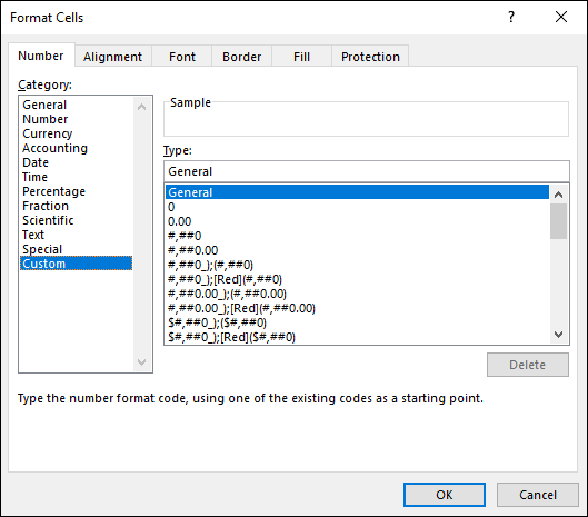
FIGURE 16-5: Formatting options in the Format Cells dialog box.

Excel lets you create custom formatting patterns so you can present your data just the way you need to. For example, you can specify whether numbers use a thousands separator, whether decimal values are always displayed to the third decimal point, and so on.

These patterns are created with the use of a few key symbols. A pound sign (#) is a placeholder for a number — that is, a single digit. Interspersing pound signs with fixed literal characters (such as a dollar sign, a percent sign, a comma, or a period) establishes a pattern. For example, this pattern — $#,###.# — says to display a dollar sign in front of the number, to use a comma for a thousands separator, and to display one digit to the right of the decimal point. Some formatting options used with the TEXT function are shown in Table 16-1. Look up custom number formatting in Excel Help for more information on custom format patterns, or go to www.microsoft.com and search for guidelines for custom number formats.

TABLE 16-1 Formatting Options for the TEXT Function

Format	Displays
=TEXT(1234.56,"#.##")	1234.56
=TEXT(1234.56,"#.#")	1234.6
=TEXT(1234.56,"#")	1235
=TEXT(1234.56,"$#")	$1235
=TEXT(1234.56,"$#,#")	$1,235
=TEXT(1234.56,"$#,#.##")	$1,234.56
=TEXT(0.4,"#%")	40%
=TEXT("3/15/2005","mm/dd/yy")	03/15/05
=TEXT("3/15/2005","mm/dd/yyyy")	03/15/2005
=TEXT("3/15/2005","mmm-dd")	Mar-15

Figure 16-6 shows how the TEXT function is used to format values that are incorporated into sentences. Column C contains the formulas that use TEXT. For example, C4 has this formula: ="We spent " & TEXT(B4,"$#,#.#0") & " on " & A4. Cell C8 has this formula: ="We opened the office on " & TEXT(B8,"mmm d, yyyy").

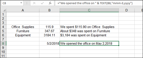
FIGURE 16-6: Using TEXT to report in a well-formatted manner.

Here's how to use TEXT:

1. Position the cursor in the cell where you want the results to appear.
2. Type =TEXT( to begin the function entry.
3. Click a cell that contains a number or a date or enter its address.
4. Enter a comma (,).

5. Enter a " and then enter a formatting pattern.

   See the Format Cells dialog box (the Custom category of the Number tab) for guidance.

6. Enter a " after the pattern is entered.
7. Type a ) and press Enter.

The VALUE function does the opposite of TEXT; it converts strings to numbers (this is not to say text such as twenty, but numbers that have been formatted as text). Excel does this by default anyway, so I don’t cover the VALUE function here. You can look it up in Excel’s Help system if you’re curious about it.

Repeating text

REPT is a nifty function that does nothing other than repeat a string of text. REPT has two arguments:

• The string or a reference to a cell that contains text
• The number of times to repeat the text

REPT makes it a breeze to enter a large number of repeating characters. Figure 16-7 shows how this works. Cells B14 and B15 contain important summary information. To make this stand out, a string of asterisks (*) has been placed above and below, respectively, in B13 and B16. The REPT function was used here, with this formula: =REPT("*",120). This simple function has removed the drudgery of having to enter 120 asterisks.

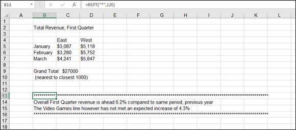
FIGURE 16-7: Repeating text with the REPT function.

Try it out:

1. Position the cursor in the cell where you want the results to appear.
2. Type =REPT( to begin the function entry.

3. Click a cell that contains text or enter text enclosed in double quotation marks.

   Typically, you would enter a character (such as a period or an asterisk), but any text will work.

4. Type a comma (,).
5. Enter a number to tell the function how many times to repeat the text.
6. Type a ) and press Enter.

Swapping text

Two functions — REPLACE and SUBSTITUTE — replace a portion of a string with other text. The functions are nearly identical in concept but are used in different situations.

Both REPLACE and SUBSTITUTE replace text within other text. Use REPLACE when you know the position of the text you want to replace. Use SUBSTITUTE when you don't know the position of the text you want to replace.

REPLACE

REPLACE takes four arguments:

• The target string as a cell reference
• The character position in the target string at which to start replacing
• The number of characters to replace
• The string to replace with (does not have to be the same length as the text being replaced)

For example, if cell A1 contains the string Our Chicago office has closed., the formula =REPLACE(A1,5,7,"Dallas") returns the string Our Dallas office has closed.

Figure 16-8 shows how to use REPLACE with the Inventory Control data first shown in the “Breaking Apart Text” section. A new task is at hand. For compatibility with a new computer system, you have to modify the product codes in the inventory data with two dashes between the vendor ID and the internal tracking number. The original codes are in column A. Use a combination of REPLACE and LEFT functions to get the job done: =REPLACE(A4, 1, 3, LEFT(A4,3) & "--").

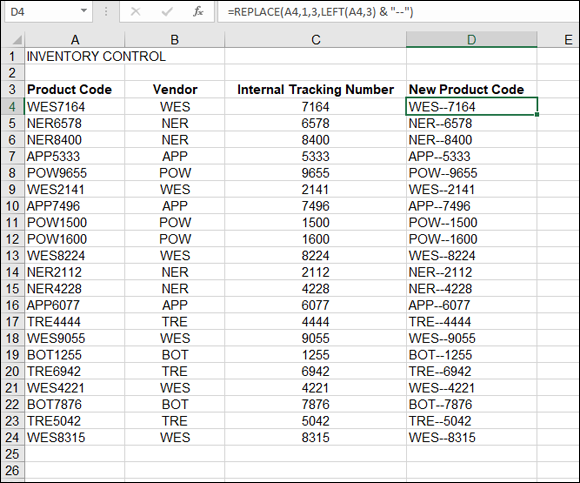
FIGURE 16-8: Using REPLACE to change text.

These arguments replace the original three characters in each product code with the same three characters followed by two dashes. Figure 16-8 shows how REPLACE alters the product codes. In the figure, the first three product code characters are replaced with themselves and the dashes. The LEFT function and the dashes serve as the fourth argument of REPLACE.

Keep in mind a couple of points about REPLACE:

• You need to know where the text being replaced is in the larger text.

  Specifically, you have to tell the function at what position the text starts and how many positions it occupies.

• The text being replaced and the new text taking its place don't have to be the same length.

Here’s how to use the REPLACE function:

1. Position the cursor in the cell where you want the result to appear.
2. Type =REPLACE( to begin the function entry.
3. Click a cell that contains the full string of which a portion is to be replaced.
4. Type a comma (,).
5. Enter a number to tell the function the starting position of the text to be replaced.
6. Type a comma (,).
7. Enter a number to tell the function how many characters are to be replaced.
8. Type a comma (,).

9. Click a cell that contains text or enter text enclosed in double quotation marks.

   This is the replacement text.

10. Type a ) and press Enter.

You can also use REPLACE to delete text from a string. Simply specify an empty string (" ") as the replacement text.

SUBSTITUTE

Use the SUBSTITUTE function when you don’t know the position in the target string of the text to be replaced. Instead of telling the function the starting position and number of characters (as you do with REPLACE), you just tell it what string to look for and replace.

SUBSTITUTE takes three required arguments and a fourth optional argument:

• A reference to the cell that contains the target text string
• The string within the target string that is to be replaced
• The replacement text
• An optional number to tell the function which occurrence of the string to replace

The fourth argument tells SUBSTITUTE which occurrence of the text to be changed (the second argument) and actually replaced with the new text (the third argument). The text to be replaced may appear more than once in the target string. If you omit the fourth argument, all occurrences are replaced. This is the case in the first example in Table 16-2; all spaces are replaced with commas. In the last example in Table 16-2, only the second occurrence of the word two is changed to the word three.

TABLE 16-2 Applying the SUBSTITUTE Function

Example	Returned String	Comment
=SUBSTITUTE("apple banana cherry fig", " ",",")	apple,banana,cherry,fig	All spaces are replaced with commas.
=SUBSTITUTE("apple banana cherry fig", " ",",",1)	apple,banana cherry fig	The first space is replaced with a comma. The other spaces remain as they are.
=SUBSTITUTE("apple banana cherry fig", " ",",",3)	apple banana cherry,fig	The third space is replaced with a comma. The other spaces remain as they are.
=SUBSTITUTE("There are two cats and two birds.","two","three")	There are three cats and three birds.	Both occurrences of two are replaced with three.
=SUBSTITUTE("There are two cats and two birds.","two","three",2)	There are two cats and three birds.	Only the second occurrence of two is replaced with three.

Try it yourself! Here's what you do:

1. Position the cursor in the cell where you want the result to appear.
2. Type =SUBSTITUTE( to begin the function entry.

3. Click a cell that contains text or enter its address.

   This is the full string of which a portion is to be replaced.

4. Type a comma (,).

5. Click a cell that contains text or enter text enclosed in double quotation marks.

   This is the portion of text that is to be replaced.

6. Type a comma (,).

7. Click a cell that contains text or enter text enclosed in double quotation marks.

   This is the replacement text. If you want to specify which occurrence of text to change, continue to steps 8 and 9; otherwise, go to Step 10.

8. Type a comma (,).
9. Enter a number that tells the function which occurrence to apply the substitution to.
10. Type a ) and press Enter.

You can use SUBSTITUTE to remove spaces from text. In the second argument (what to replace), enter a space enclosed in double-quote marks. In the third argument, enter two double-quote marks with nothing between them. This is known as an empty string.

Giving text a trim

Spaces have a way of sneaking in and ruining your work. The worst thing is that you often can’t even see them! When the space you need to remove is at the beginning or end of a string, use the TRIM function to remove them. The function simply clips any leading or trailing spaces from a string. It also removes extra spaces from within a string; a sequence of two or more spaces is replaced by a single space.

Figure 16-9 shows how this works. In column A is a list of names. Looking closely, you can see that some unwanted spaces precede the names in cells A5 and A10. Column B shows the correction using TRIM. Here is the formula in cell B5: =TRIM(A5).

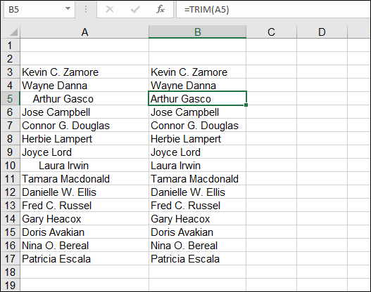
FIGURE 16-9: Removing spaces with the TRIM function.

TRIM takes just one argument: the text to be cleaned of leading and trailing spaces. Here’s how it works:

1. Position the cursor in the cell where you want the result to appear.
2. Type =TRIM( to begin the function entry.
3. Click a cell that contains the text that has leading or trailing spaces, or enter the cell address.
4. Type a ) and press Enter.

Be on the lookout: Although you generally use it to remove leading and trailing spaces, TRIM removes extra spaces in the middle of a string. If two or more spaces are next to each other, TRIM removes the extra spaces and leaves one space in place.

This is usually a good thing. Most times, you don’t want extra spaces in the middle of your text. But what if you do? Here are a couple of alternatives to remove a leading space, if it is there, without affecting the middle of the string:

Formula to Remove Leading Space	Comment
=IF(LEFT(E10,1)=" ",SUBSTITUTE(E10," ","",1), E10)	If a space is found in the first position, substitute it an empty string; otherwise, just return the original string.
=IF(LEFT(E10,1)=" ",RIGHT(E10,LEN(E10)-1), E10)	If a space is found in the first position, return the right side of the string, less the first position. (See the section on LEN, earlier in this chapter.)

Making a case

In school, you were taught to use an uppercase letter at the start of a sentence as well as for proper nouns. But that was a while ago, and now the brain cells are a bit fuzzy. Lucky thing Excel has a way to help fix case, er Case, um CASE — well, you know what I mean.

Three functions alter the case of text: UPPER, LOWER, and PROPER. All three functions take a single argument — the text that will have its case altered. Here are a few examples:

Formula	Result
=LOWER("The Cow Jumped Over The Moon")	the cow jumped over the moon
=UPPER("the cow jumped over the moon")	THE COW JUMPED OVER THE MOON
=PROPER("the cow jumped over the moon")	The Cow Jumped Over The Moon

Try this:

1. Enter a sentence in a cell.

   Any old sentence will do, but don’t make any letters uppercase. For example, type excel is great or computers give me a headache.

2. Position the cursor in an empty cell.
3. Type =UPPER( to start the function.
4. Click the cell that has the sentence or enter its address.
5. Type a ) and press Enter.
6. In another empty cell, type =PROPER( to start the function.
7. Click the cell that has the sentence or enter its address.

8. Type a ) and press Enter.

   You should now have two cells that show the sentence with a case change. One cell has the sentence in uppercase; the other cell, in proper case.

Perhaps you noticed another possibility that needs to be addressed. What about when just the first word needs to start with an uppercase letter and the rest of the string is all lowercase? Some people refer to this as sentence case. You can create sentence case by using the UPPER, LEFT, RIGHT, and LEN functions. (LEN is explained earlier in this chapter.) With the assumption that the text is in cell B10, here is how the formula looks:

=UPPER(LEFT(B10,1)) & RIGHT(B10,LEN(B10)-1)

In a nutshell, the UPPER function is applied to the first letter, which is isolated with the help of the LEFT function. This result is concatenated with the remainder of the string. You know how much is left by using LEN to get the length of the string and using the RIGHT function to get all the characters from the right, less one. This type of multi-use function work takes a bit of getting used to.

Comparing, Finding, and Measuring Text

Excel has many functions that manipulate text, but sometimes you just need to find out about the text before you do anything else! A handful of functions determine whether text matches other text, let you find text inside other text, and tell you how long a string is. These functions are passive — that is, they do not alter text.

Going for perfection with EXACT

The EXACT function lets you compare two strings of text to see whether they’re the same. The function takes two arguments — the two strings of text — and returns a true or false value. EXACT is case sensitive, so two strings that contain the same letters but with differing case produce a result of false. For example, Apple and APPLE are not identical.

EXACT is great for finding changes in data. Figure 16-10 shows two lists of employees, one for each year, in columns A and B. Are they identical? You could spend a number of minutes staring at the two lists. (That would give you a headache!) Or you can use EXACT. The cells in column C contain the EXACT function, used to check column A against column B. The returned values are true for the most part. This means there is no change.

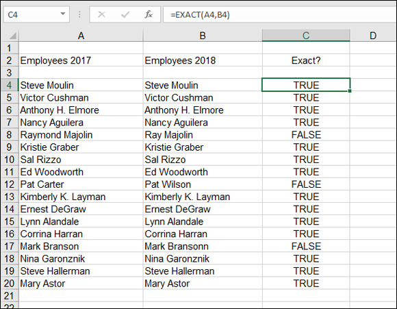
FIGURE 16-10: Comparing strings with the EXACT function.

A few names are different in the second year. Marriage, divorce, misspellings — the mismatched data could be any of these. EXACT returns false for these names, which means they aren't identical in the two lists and should be checked manually.

Here’s how you use EXACT:

1. Position the cursor in the cell where you want the results to appear.
2. Type =EXACT( to begin the function entry.
3. Click a cell that contains text or enter its address.
4. Type a comma (,).
5. Click another cell that has text or enter its address.
6. Type a ) and press Enter.

If you get a true result with EXACT, the strings are identical. A false result means they’re different.

What if you want to compare strings without regard to case? In other words, APPLE and apple would be considered the same. Excel does not have a function for this, but the result is easily obtained with EXACT and UPPER. The idea is to convert both strings to uppercase and compare the results:

=EXACT(UPPER("APPLE"), UPPER("apple"))

You could just as well use LOWER here.

Finding and searching

Two functions, FIND and SEARCH, work in a quite similar fashion. A couple of differences are key to figuring out which to use. Both FIND and SEARCH find one string inside a larger string and tell you the position at which it was found (or produce #VALUE if it is not found). The differences follow:

FIND	SEARCH
Case-sensitive. It will not, for example, find At inside heat.	Not case-sensitive.
You cannot use the wildcards * and ?.	You can use the wildcards * and ?.

FIND

FIND takes three arguments:

• The string to find
• The larger string to search in
• The position in the larger string to start looking at; this argument is optional

If the third argument is left out, the function starts looking at the beginning of the larger string. Here are some examples:

Value in Cell A1	Function	Result
Happy birthday to you	=FIND("Birthday",A1)	#VALUE!
Happy birthday to you	=FIND("birthday",A1)	7
Happy birthday to you	=FIND("y",A1)	5
Happy birthday to you	=FIND("y",A1,10)	14

In the first example using FIND, an error is returned. The #VALUE! error is returned if the text cannot be found. Birthday is not the same as birthday, at least to the case-sensitive FIND function.

SEARCH

The SEARCH function takes the same arguments as FIND. The two common wildcards you can use are the asterisk (*) and the question mark (?). An asterisk tells the function to accept any number of characters (including zero characters). A question mark tells the function to accept any single character. It is not uncommon to see more than one question mark together as a wildcard pattern. Table 16-3 shows several examples.

TABLE 16-3 Using the SEARCH Function

Value in Cell A1	Function	Result	Comment
Happy birthday to you	=SEARCH("Birthday",A1)	7	birthday starts in position 7.
Happy birthday to you	=SEARCH("y??",A1)	5	The first place where a y is followed by any two characters is at position 5. This is the last letter in Happy, a space, and the first letter in birthday.
Happy birthday to you	=SEARCH("yo?",A1)	19	The first place where yo is followed by any single character is the word you.
Happy birthday to you	=SEARCH("b*d",A1)	7	The search pattern is the letter b, followed by any number of characters, followed by the letter d. This starts in position 7.
Happy birthday to you	=SEARCH("*b",A1)	1	The asterisk says search for any number of characters before the letter b. The start of characters before the letter b is at position 1. Using an asterisk at the start is not useful. It will either return a 1 or an error if the fixed character(s) (the letter b in this example) is not in the larger text.
Happy birthday to you	=SEARCH("t*",A1)	10	The asterisk says search for any number of characters after the letter t. Because the search starts with a fixed character, its position is the result. The asterisk serves no purpose here.
Happy birthday to you	=SEARCH("t",A1,12)	16	Finds the position of the first letter t, starting after position 12. The result is the position of the first letter in the word to. The letter t in birthday is ignored.

Back in Figure 16-3, I show you how to concatenate first and last names. What if you have full names to separate into first names and last names? SEARCH to the rescue! (Does that make this a search-and-rescue mission?) Figure 16-11 shows how the SEARCH, LEFT, RIGHT, and ISERROR functions work together to turn names into individual first and last names.

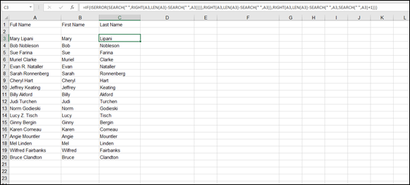
FIGURE 16-11: Splitting names apart.

Isolating the first name from a full name is straightforward. You just use LEFT to get characters up to the first space. The position of the first space is returned from the SEARCH function. Here is how this looks:

=LEFT(A3,SEARCH(" ",A3)-1)

Getting the last names is just as simple — not! When the full name has only first and last names (no middle name or initials), you need SEARCH, RIGHT, and LEN, like this:

=RIGHT(A3,LEN(A3)-SEARCH(" ",A3))

However, this does not work for middle names or initials. What about Franklin D. Roosevelt? If you rely on the last name’s being after the first space, the last name becomes D. Roosevelt. An honest mistake, but you can do better. What you need is a way to test for the second space and then return everything to the right of that space. There are likely a number of ways to do this.

Here is what you see in column C, in Figure 16-11:

=IF(ISERROR(SEARCH(" ",RIGHT(A3,LEN(A3)-SEARCH(" ",A3)))),RIGHT(A3,LEN(A3)-SEARCH(" ",A3)),RIGHT(A3,LEN(A3)-SEARCH(" ",A3,SEARCH(" ",A3)+1)))

Admittedly, it’s a doozy. But it gets the job done. Here is an overview of what this formula does:

• It’s an IF function and therefore tests for either true or false.
• The test is if an error is returned from SEARCH for trying to find a space to the right of the first space:

  ISERROR(SEARCH(" ",RIGHT(A3,LEN(A3)-SEARCH(" ",A3))))

• If the test is true, there is no other space. This means there is no middle initial, so just return the portion of the name after the first space:

  RIGHT(A3,LEN(A3)-SEARCH(" ",A3))

• If the test is false, there is a second space, and the task is to return the portion of the string after the second space. SEARCH tells both the position of the first space and the second space. This is done by nesting one SEARCH inside the other. The inner SEARCH provides the third argument — where to start looking from. A 1 is added so the outer SEARCH starts looking for a space one position after the first space:

  RIGHT(A3,LEN(A3)-SEARCH(" ",A3,SEARCH(" ",A3)+1))

Your eyes have probably glazed over, but that’s it!

The monster formula isolates last names from full names that include a middle initial. A task for you to try, if you have any working brain cells left, is to write a formula that isolates the middle initial, if there is one. Here’s how to use FIND or SEARCH:

1. Position the cursor in the cell where you want the results to appear.
2. Type =FIND( or =SEARCH( to begin the function entry.
3. Enter a string of text that you want in a larger string, enclosed with double quotation marks, or click a cell that contains the text.
4. Type a comma (,).

5. Click a cell that contains the larger text or enter its address.

   If you want the function to begin searching at the start of the larger string, go to Step 7. If you want to have the function begin the search in the larger string at a position other than 1, go to Step 6.

6. Type a comma (,) and the position number.
7. Type a ) and press Enter.