Chapter 17
Playing Records with Database Functions
IN THIS CHAPTER
 Understanding an Excel database structure
Figuring out how criteria work
Adding, averaging, and counting database records
Testing for duplicate records
Believe it or not, an Excel worksheet has the same structure as a database table. A database table has fields and records; an Excel worksheet has columns and rows. Same thing. Given this fact, why not ask questions of, or query, your information in much the same way as you do with a database?
In this chapter, I tell you how to use Excel’s database functions to get quick answers from big lists. Say you have a client list on a worksheet — name, address, that sort of thing. You want to know how many clients are in New York. You may think about sorting your list by state and then counting the number of rows. Forget it. That’s the old way! In this chapter, I show you how to do this sort of thing with a single function.
Putting Your Data into a Database Structure
 To use the database functions, you need to put your data into a structured format. Excel is very flexible. Usually, you put data wherever you want. But to make the best of the database functions, you need to get your data into a contiguous area of rows and columns. Each row is a record, and each column is a field. The top row contains labels that identify the fields.
Figure 17-1 shows a database in a worksheet. This example is a list of students (by ID number) and their classes, teachers, and grades. Each student occupies a row — in other words, a record — in the database. Each of the four fields — Student ID, Class, Teacher, and Final Grade — is in one column and is identified by a label in the top row.
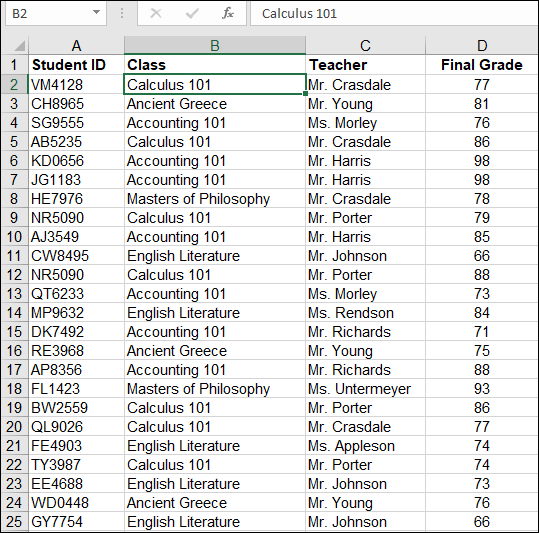
FIGURE 17-1: Using a database to store student information.
The data in the worksheet in Figure 17-1 is really just normal data. There is nothing special about it. However, the data sits in organized rows and columns, making it ready for working with Excel’s database functions:
- Each column is a field that holds one particular item of data, such as Student ID or Class. It must contain no other data.
- Each row contains one record. In this example, a record is the data for one student.
- The top row of the database contains labels that identify the fields.
This sample data is used in this chapter to demonstrate the database functions. Of course, you can have a database in Excel and never use the database functions, but you have a lot more power at your fingertips if you do use them.
Working with Database Functions
The database functions all work in basically the same way. They perform some calculation on a specified field for those records that meet specified criteria. For example, you can use a database function to calculate the average final grade for all students in Accounting 101.
All database functions use the following three arguments:
- The database range: This argument tells the function where the database is. You enter it by using cell addresses (for example, A1:D200) or a named range (for example, Students). The range must include all records, including the top row of field names.
- The field: You must tell a database function which field to operate on. You can’t expect it to figure this out by itself! You can enter either the column number or the field name. A column number, if used, is the number of the column offset from the first column of the database area. In other words, if a database starts in column C, and the field is in column E, the column number is 3, not 5. If a heading is used, put it inside a set of double quotation marks. Database functions calculate a result based on the values in this field. Just how many values are used depends on the third argument: the criteria.
- The criteria: This tells the function where the criteria are located; it is not the criteria per se. The criteria tell the function which records to use in its calculation. You set up the criteria in a separate part of the worksheet, apart from the database area. This area’s address is passed to the database function. Criteria are explained in detail throughout the chapter.
Establishing your database
All database functions take a database reference as the first argument. The database area must include headers (field names) in the first row. In Figure 17-1 earlier in this chapter, the first row uses Student ID, Class, Teacher, and Final Grade as headers to the information in each respective column.
 A great way to work with the database functions is to name the database area and then enter the name, instead of the range address, in the function.
To set up a name, follow these steps:
Select the entire database area.
Make sure the top row has headers and is included in the selection.
- Click the Formulas tab (at the top of the Excel window).
Click Define Name in the Defined Names area.
The New Name dialog box appears, with the range address set in the Refers To box.
- Type a name in the Name Box (or use the suggested name).
- Click OK to close the dialog box.
Later, if records are added to the bottom of the database, you have to redefine the named area’s range to include the new rows. You can do this as follows:
Click the Name Manager button on the Excel Formulas tab.
The Name Manager dialog box appears.
- Click the name in the list you want to redefine.
Click the Edit button in the dialog box.
Excel opens the Edit Name dialog box, shown in Figure 17-2, with information about the selected range.
Change the reference in the Refers To box.
You can use the small square button to the right of the Refers To box to define the new reference by dragging the mouse pointer over it. Clicking the small square button reduces the size of the Edit Name dialog box and allows you access to the worksheet. When you are done dragging the mouse over the new worksheet area, press Enter to get back to the Edit Name dialog box.
- Click OK to save the reference change and close the dialog box.
- Click Close.
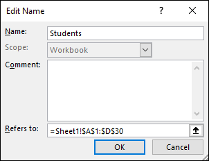
FIGURE 17-2: Updating the reference to a named area.
If you add records to your database range by inserting new rows somewhere in the middle, rather than adding them on at the end, Excel automatically adjusts the reference to the named range.
Establishing the criteria area
As I mention earlier, the criteria are not part of the database function arguments but are somewhere in the worksheet and then referenced by the function. The criteria area can contain a single criterion, or it can contain two or more criteria. Each individual criterion is structured as follows:
- In one cell, enter the field name (header) of the database column that the criterion will apply to.
- In the cell below, enter the value that the field data must meet.
Figure 17-3 shows the student database with a criteria area to the right of the database. There are places to put criteria for the Class, Teacher, and Final Grade. In the example, a criterion has been set for the Class field. This criterion forces the database function to process only records (rows) where the Class is Accounting 101. Note, though, that a criterion can be set for more than one field. In this example, the Teacher and Final Grade criteria have been left blank so they don’t affect the results.
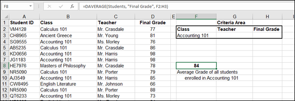
FIGURE 17-3: Selecting criteria to use with a database function.
The DAVERAGE function has been entered into cell F8 and uses this criteria range. The three arguments are in place. The name Students tells the function where the database is, the Final Grade field (column) is where the function finds values to calculate the average, and the criteria are set to the worksheet range that has criteria that tell the function to use only records where the Class is Accounting 101 — in other words, F2:H3. The entry in cell F8 looks like this:
=DAVERAGE(Students,"Final Grade",F2:H3)
Why does this function refer to F2:H3 as the criteria range when the only defined criterion is located in the range F2:F3? It’s a matter of convenience. Because cells G3 and H3 in the criteria range are blank, the Teacher and Final Grade fields are ignored by a database function that uses this criteria range. However, if you want to enter a criterion for one of those fields, just enter it in the appropriate cell; there is no need to edit the database function arguments. What about assigning a name to the criteria area and then using the name as the third argument to the database function? That works perfectly well, too.
 Whether you use a named area for your criteria or simply type the range address, you must be careful to specify an area that includes all the criteria but does not include any blank rows or columns. If you do, the database function’s results will be incorrect.
Here’s how you enter any of the database functions. This example uses the DSUM function, but the instructions are the same for all the database functions; just use the one that performs the desired calculation. Follow these steps:
Import or create a database of information in a worksheet.
The information should be in contiguous rows and columns. Be sure to use field headers.
Optionally, use the New Name dialog box to give the database a name.
To name your database, see the section “Establishing your database” earlier in this chapter.
Select a portion of the worksheet to be the criteria area and then add headers to this area that match the database headers.
You have to provide criteria headers only for database fields that criteria are applied to. For example, your database area may have ten fields, but you need to define criteria to three fields. Therefore, the criteria area can be three columns wide.
Position the cursor in the cell where you want the results to appear.
This cell must not be in the database area or the criteria area.
- Type =DSUM( to begin the function entry.
- Enter the database range or a name, if one is set.
- Type a comma (,).
- Enter either of the following:
- The header name, in quotation marks, of the database field that the function should process
- The column number
- Type a comma (,).
- Enter the range of the criteria area.
- Type a ) and press Enter.
Fine-Tuning Criteria with AND and OR
Excel’s database functions would not be of much use if you could not create fairly sophisticated queries. A few common types of queries follow:
- Records that match two or more individual criteria
- Records that match any one of several criteria
- Values that fall within a specified range of values
To find records that match two or more criteria, place the criteria in adjacent columns in the criteria area. Continuing with the student-grade database, the criteria area shown in Figure 17-4 matches records where the Class field contains Accounting 101 and the Teacher field contains Mr. Harris. This is called an AND criterion.
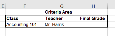
FIGURE 17-4: Finding records that match two criteria.
To match records that meet any one of several criteria, place the individual criteria in two or more rows below the field name. Figure 17-5 shows a criteria range that matches all records where the Class field contains either Accounting 101 or English Literature. This is called an OR criterion.
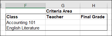
FIGURE 17-5: Finding records that match any one of two or more criteria.
To combine AND with OR in a criteria range, use two or more columns and two or more rows. Figure 17-6 shows a criteria range that finds all records where Class is Accounting 101 and Teacher is either Mr. Harris or Mr. Richards.
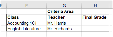
FIGURE 17-6: Combining AND and OR criteria.
To define a criterion that uses ranges of values, use these numerical comparison operators:
- < for less than
- > for greater than
- <= for less than or equal to
- >= for greater than or equal to
Of course, you can apply these to fields with numerical values. Figure 17-7 shows two criteria areas. The upper one matches all records in which Final Grade is 90 or higher. The lower one matches all records in which Final Grade is equal to or greater than 80 and less than 90.
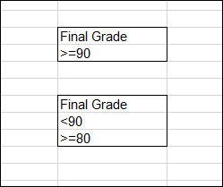
FIGURE 17-7: Defining numerical range criteria.
Adding Only What Matters with DSUM
The DSUM function lets you sum numbers in a database column for just those rows that match the criteria you specify. For example, take a database that contains data on individual sale amounts for sales people. The database range is named Sales. You want to calculate total sales for each of the three sales representatives. Figure 17-8 shows how this is done. Three criteria areas are defined in D2:D3, E2:E3, and F2:F3. The DSUM function is entered in cells E8:E10. The formula in cell E8 is
=DSUM(SALES, "Sale Amount", D2:D3)
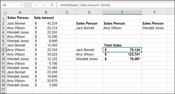
FIGURE 17-8: Calculating the sum of sales with the DSUM function.
The functions entered in E9 and E10 are identical except for referencing a different criteria range. The results show clearly that Amy is the sales leader.
Going for the Middle with DAVERAGE
The DAVERAGE function lets you find the average, or mean, of a field for just the rows that match the criteria. For this example, you return to the student database.
Figure 17-9 shows a worksheet in which the average grade for each course has been calculated by DAVERAGE. For example, cell G22 shows the average grade for Masters of Philosophy. Here is the formula:
=DAVERAGE(Students,"Final Grade",F14:G15)

FIGURE 17-9: Calculating the average grade for each course.
Each calculated average uses a different criteria area. Each area filters the result by a particular course. In all cases, the criteria area for the Teacher is left blank and, therefore, has no effect on the results.
For the sake of comparison, DAVERAGE is also used in cell G24 to show the overall average for all courses. Because a criterion is a required function argument, the calculation in cell G24 is set to look at an empty cell. None of the Class criteria cells is free, so the function looks to the Teacher criterion in cell G3. Because this cell has no particular teacher entered as a criterion, all of the records in the database are used to create this average — just what you want. Here is the formula in cell G24:
=DAVERAGE(Students,"Final Grade",G2:G3)
It doesn't matter which field header you use in the criterion when you’re getting a result based on all records in a database. What does matter is that there is no actual criterion below the header.
Counting Only What Matters with DCOUNT
The DCOUNT function lets you determine how many records in the database match the criteria.
Figure 17-10 shows how DCOUNT can determine how many students took each course. Cells G18:G22 contain formulas that count records based on the criterion (the Class) in the associated criteria sections. Here is the formula used in cell G20, which counts the number of students in Calculus 101:
=DCOUNT(Students,"Final Grade",F8:G9)
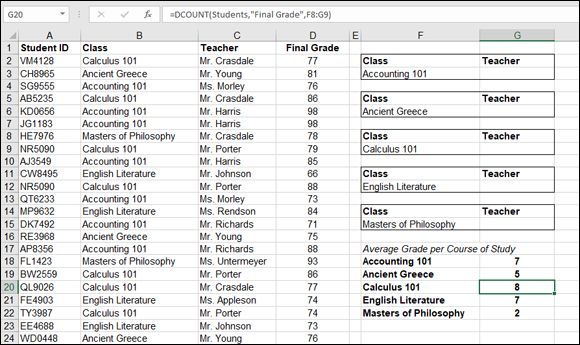
FIGURE 17-10: Calculating the number of students in each course.
Note that DCOUNT requires a column of numbers to count. Therefore, the Final Grade heading is put in the function. Counting on Class or Teacher would result in zero. Using a column that specifically has numbers may seem a little odd. The function is not summing the numbers; it just counts the number of records. But what the heck? It works.
Now take this a step further. How about counting the number of students who got a grade of 90 or better in any class? How can this be done? This calculation requires a different criterion — one that selects all records where Final Grade is 90 or greater. Figure 17-11 shows a worksheet with this criterion and the calculated result shown.
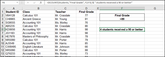
FIGURE 17-11: Calculating the number of students who earned a grade of 90 or better.
The result in cell F6 concatenates — that is, combines but does not add — the answer from the DCOUNT function with some text. The formula looks like this:
=DCOUNT(Students,"Final Grade",F2:F3) & " students received a 90 or better."
The criterion specifically states to use all records where the Final Grade is greater than 89 (>89). You can specify >=90 with the exact same result.
Finding Highest and Lowest with DMIN and DMAX
The DMIN and DMAX functions find the minimum or maximum value, respectively, in a database column, for just the rows that match the criteria. Figure 17-12 shows how these two functions can find the highest and lowest grades for English Literature.
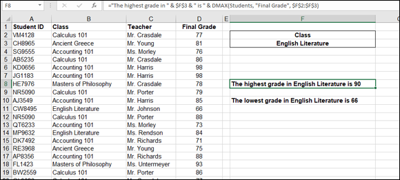
FIGURE 17-12: Calculating the highest and lowest grades for a specified class.
The formulas in cells F8 and F10 are practically identical. Here is the formula in cell F8:
="The highest grade in " & $F$3 & " is " & DMAX(Students,"Final Grade",$F$2:$F$3)
Finding Duplicate Values with DGET
DGET is a unique database function. It does not perform a calculation but checks for duplicate entries. The function returns one of three values:
- If one record matches the criterion, DGET returns the criterion.
- If no records match the criterion, DGET returns the
#VALUE!error. - If more than one record matches the criterion, DGET returns the
#NUM!error.
By testing to see whether DGET returns an error, you can discover problems with your data. Perhaps you suspect that a student has registered twice for a specific class. If this is true, two records will have the same Student ID and Class.
Figure 17-13 shows how to check whether student NR5090 is entered more than once for Calculus 101. If there is more than one record, DGET returns an error. Cell F5 contains a formula that nests the DGET function inside the ISERROR function; all that is inside the IF function. If DGET returns an error, return one message; if DGET does not return an error, return a different message. Here is the formula:
=IF(ISERROR(DGET(Students,"Student ID",F2:G3)),F3 & " has duplicate records", F3 & " has one record")
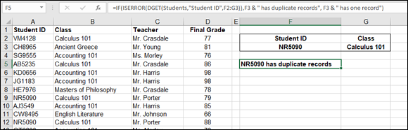
FIGURE 17-13: Using DGET to test for duplicate records in a database.
Being Productive with DPRODUCT
DPRODUCT multiplies values that match the criterion in a database. This is powerful but also able to produce results that are not the intention. In other words, it's one to thing to add and derive a sum. That is a common operation on a set of data. Looking back at Figure 17-8, you can see that the total sales for Jack Bennet, $79,134, are the sum of three amounts: $43,234, $12,450, and $23,450. If multiplication were applied to the three amounts, the answer (the product) would be $12,622,274,385,000. Oops! That's over 12 trillion dollars!
DPRODUCT multiplies and, therefore, is not likely to be used as often as a function like DSUM, but when you need to multiply items in a database, DPRODUCT is a tool of choice.
Figure 17-14 shows a situation in which DPRODUCT is productive. The database area contains shirts. For each shirt size, there are two rows: the price per shirt and the number of shirts that are packed in a carton. The cost for a carton of shirts is, therefore, the product of the price per shirt times the number of shirts. There are four shirt sizes, each with its own price and carton count.
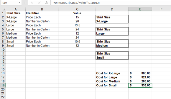
FIGURE 17-14: Calculating the total costs of cartons filled with shirts.
To make sure you work with just one size per use of DPRODUCT, four criteria areas are set up — one for each size. Any single criteria area has the Shirt Size heading and the actual shirt size, such as Medium. For example, D8:D9 contains the criteria for medium-size shirts.
Four cells each contain DPRODUCT, and within each cell, the particular criteria area is used. For example, cell E18 has this formula:
=DPRODUCT(A1:C9, "Value", D8:D9)
The database range is A1:C9. Value is the field the function looks in for values to multiply, and the multiplication occurs on values for which the shirt size matches the criteria.
A worksheet set up like the one shown in Figure 17-14 is especially useful when new data are occasionally pasted into the database area. The set of DPRODUCT functions will always provide the products based on whatever data are placed in the database area. This particular example of DPRODUCT shows how to work with data in which more than one row pertains to an item. In this case, each shirt size has a row showing the price per shirt and a second row showing the number of shirts that fit in a carton.