Chapter 18

Ten Tips for Working with Formulas

IN THIS CHAPTER

Making sure the order of operators is correct

Viewing and fixing formulas

Referencing cells and using names

Setting the calculation mode

Using conditional formatting and data validation

Writing your own functions

Several elements can help you be as productive as possible when writing and correcting formulas. You can view all your formulas at once and correct errors one by one. You can use add-in wizards to help write functions. You can even create functions all on your own!

Master Operator Precedence

One of the most important factors in writing formulas is getting the operators correct, and I do not mean telephone-company operators. This has to do with mathematical operators — you know, little details such as plus signs, and multiplication signs, and where the parentheses go. Operator precedence — the order in which operations are performed — can make a big difference in the result. You have an easy way to keep your operator precedence in order. All you have to remember is “Please excuse my dear Aunt Sally.”

No, I have not lost my mind! This phrase is a mnemonic for the following:

• Parentheses
• Exponents
• Multiplication
• Division
• Addition
• Subtraction

Thus, parentheses have the first (highest) precedence, and subtraction has the last precedence. Well, to be honest, multiplication has the same precedence as division and addition has the same precedence as subtraction, but you get the idea!

For example, the formula =1 + 2 × 15 equals 31. If you think it should equal 45, you'd better go visit your aunt! The answer equals 45 if you include parentheses, such as this: =(1 + 2) × 15.

Getting the order of the operators correct is critical to the well-being of your worksheet. Excel generates an error when the numbers of open and closed parentheses do not match, but if you mean to add two numbers before the multiplication, Excel does not know that you simply left the parentheses out!

A few minutes of refreshing your memory on operator order can save you a lot of headaches down the road.

Display Formulas

In case you haven’t noticed, it’s kind of hard to view your formulas without accidentally editing them. That’s because any time you are in “edit” mode and the active cell has a formula, the formula may incorporate the address of any other cell you click. This totally messes things up.

Wouldn’t it be easy if you could just look at all your formulas? There is a way! It’s simple. Click File at the top left of the Excel workspace, click Options, click the Advanced tab, and then scroll down to the Display options for this worksheet section (see Figure 18-1).

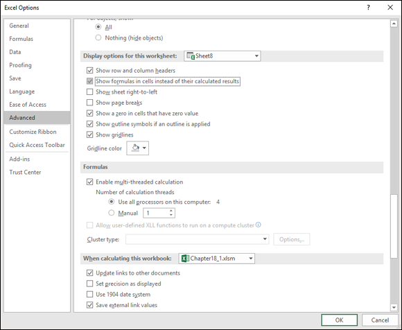
FIGURE 18-1: Setting options.

Notice the Show Formulas in Cells Instead of Their Calculated Results check box. This box tells Excel that for any cells that have formulas to display the formula itself instead of the calculated result. Figure 18-2 shows a worksheet that displays the formulas. To return to normal view, repeat these steps and deselect the option. This option makes it easy to see what all the formulas are!

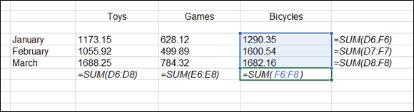
FIGURE 18-2: Viewing formulas the easy way.

You can accidentally edit functions even when you have selected the Show Formulas option. Be careful clicking around the worksheet.

Fix Formulas

Suppose that your worksheet has some errors. Don’t panic! It happens to even the savviest users, and Excel can help you figure out what’s going wrong. On the Formulas tab in the Formula Auditing section is the Error Checking button. Clicking the button displays the Error Checking dialog box, shown in Figure 18-3. That is, the dialog box appears if your worksheet has any errors. Otherwise, it just pops up a message that the error check is complete. It’s that smart!

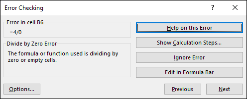
FIGURE 18-3: Checking for errors.

When there are errors, the dialog box appears and sticks around while you work on each error. The Next and Previous buttons let you cycle through all the errors before the dialog box closes. For each error it finds, you choose what action to take:

• Help on This Error: This leads to the Help system and displays the topic for the particular type of error.
• Show Calculation Steps: The Evaluate Formula dialog box opens, and you can watch step by step how the formula is calculated. This lets you identify the particular step that caused the error.
• Ignore Error: Maybe Excel is wrong. Ignore the apparent error.
• Edit in Formula Bar: This is a quick way to fix the formula yourself if you don’t need any other help.

The Error Checking dialog box also has an Options button. Clicking the button opens the Formulas tab of the Excel Options dialog box. On the Formulas tab, you can select settings and rules for how errors are recognized and triggered.

Use Absolute References

If you are going to use the same formula for a bunch of cells, such as those going down a column, the best method is to write the formula once and then drag it down to the other cells by using the fill handle. The problem is that when you drag the formula to new locations, any relative references change.

Often, this is the intention. When there is one column of data and an adjacent column of formulas, typically, each cell in the formula column refers to its neighbor in the data column. But if the formulas all reference a cell that is not adjacent, the intention usually is for all the formula cells to reference an unchanging cell reference. Get this to work correctly by using an absolute reference to the cell.

To use an absolute reference to a cell, use the dollar sign ($) before the row number, before the column letter, or before both. Do this when you write the first formula, before dragging it to other cells, or you will have to update all the formulas.

For example, don’t write this:

=A4 × (B4 + A2)

Write it this way instead:

=A4 × (B4 + $A$2)

This way, all the formulas reference A2 no matter where you copy them, instead of that reference turning into A3, and A4, and so on.

You can cycle through relative, missed, and absolute references. Press F4 to use this shortcut.

Turn Calc On/Turn Calc Off

The Excel default is to calculate your formulas automatically as they are entered or when you change the worksheet. In some situations, you may want to set the calculation to manual. Leaving the setting on automatic is usually not an issue, but if you are working on a hefty workbook with lots of calculations, you may need to rethink this one.

Imagine this: You have a cell that innocently does nothing but display the date. But dozens of calculations throughout the workbook reference that cell. Then dozens more calculations reference the first batch of cells that reference the cell with the data. Get the picture? In a complex workbook, there could be a lot of calculating going on, and the time it takes can be noticeable.

Turning the calculation setting to manual lets you decide when to calculate. Do this in the Excel Options dialog box; click the File tab on the Ribbon and then click Options. In the dialog box, click the Formulas tab, in which calculation options are selected, as shown in Figure 18-4. You can select one of the automatic calculation settings or manual calculation.

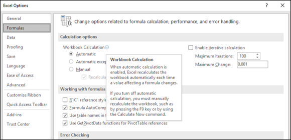
FIGURE 18-4: Setting the calculation method.

Pressing F9 calculates the workbook. Use it when the calculation is set to Manual. Here are some further options:

What You Press	What You Get
F9	Calculates formulas that have changed since the last calculation, in all open workbooks.
Shift+F9	Calculates formulas that have changed since the last calculation, just in the active worksheet.
Ctrl+Alt+F9	Calculates all formulas in all open workbooks, regardless of when they were last calculated.
Calculate Now	This is a button in the Calculation group in the Formulas tab. It calculates formulas that have changed since the last calculation, in all open workbooks.

Use Named Areas

Heck, maybe it’s just me, but I think it is easier to remember a word such as Customers or Inventory or December than it is to remember B14:E26 or AF220:AR680. So I create names for the ranges that I know I’ll reference in my formulas and functions.

Naming areas is easy to do, and in fact, you can do it a few ways. The first is to use the New Name dialog box. You can get to this by clicking the Define Name button on the Formulas tab of the Ribbon. In the dialog box, you set a range, give it a name, enter an optional comment, and then click OK (see Figure 18-5). The comment feature is useful for further notes about the range. For example, the name of the range might be “July Sales,” and in the comment area you can enter any further related information.

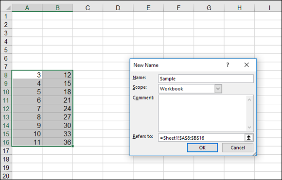
FIGURE 18-5: Defining a named area.

The Name Manager is another dialog box that you can display by clicking its button on the Formulas tab. This dialog box lets you add, update, and delete named areas. A really quick way to just add them (but not update or delete) is to follow these steps:

1. Select an area on the worksheet.

2. Click the Name Box and enter the name.

   The Name Box is part of the Formula Bar and sits to the left of where formulas are entered.

3. Press Enter.

Done! Now you can use the name as you please. Figure 18-6 shows a name being entered in the Name Box. Of course, you can use a particular name only once in a workbook. After the defined name is entered, you can find it in the Name Box by clicking the down arrow in the right of the box.

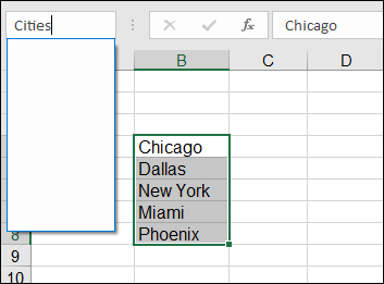
FIGURE 18-6: Defining a named area the easy way.

Use Formula Auditing

There are precedents and dependents. There are external references. There is interaction everywhere. How can you track where the formula references are coming from and going to?

Use the formula auditing tools, that’s how! On the Formulas tab is the Formula Auditing section. In the section are various buttons that control the visibility of auditing trace arrows (see Figure 18-7).

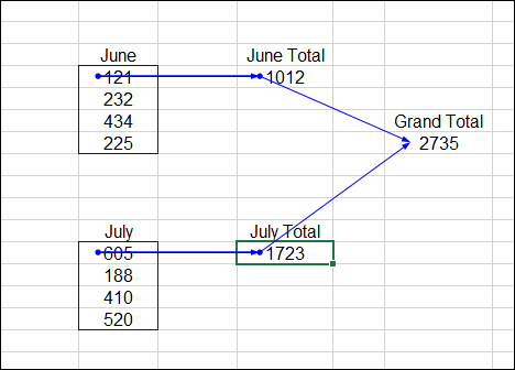
FIGURE 18-7: Auditing formulas.

The formula auditing toolbar has several features that let you wade through your formulas. Besides showing tracing arrows, the toolbar also lets you check errors, evaluate formulas, check for invalid data, and add comments to worksheets.

Use Conditional Formatting

Just as the IF function returns a certain value when the first argument condition is true and another value when it’s false, conditional formatting lets you apply a certain format to a cell when a condition is true. On the Home tab in the Styles section is a drop-down menu with many conditional formatting options. Figure 18-8 shows some values that have been treated with conditional formatting. Conditional formatting lets you set the condition and select the format that is applied when the condition is met. For example, you could specify that the cell be displayed in bold italic when the value it contains is greater than 100.

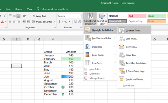
FIGURE 18-8: Applying a format when a condition is met.

Conditions are set as rules. The Rule Types are

• Format all cells based on their values.
• Format only cells that contain… .
• Format only top or bottom ranked values.
• Format only values that are above or below average.
• Format only unique or duplicate values.
• Use a formula to determine which cells to format.

When the condition is true, formatting can control the following:

• Borders
• Number formatting
• Font settings (style, color, bold, italic, and so on)
• Fill (a cell’s background color or pattern)

Cells can also be formatted with color schemes or icon images placed in the cell.

Use Data Validation

On the Data tab, in the Data Tools section, is Data Validation. Data Validation lets you apply a rule to a cell (or a range of cells) that the entry must adhere to. For example, a cell can be set to accept only an integer entry between 50 and 100 (see Figure 18-9).

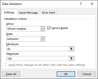
FIGURE 18-9: Setting data validation.

When entry does not pass the rule, a message is displayed (see Figure 18-10).

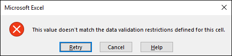
FIGURE 18-10: Caught making a bad entry.

The error message can be customized. For example, if someone enters the wrong number, the displayed error message can say Noodlehead — learn how to count! Just don't let the boss see that.

Create Your Own Functions

Despite all the functions provided by Excel, you may need one that you just don’t see offered. Excel lets you create your own functions by using VBA programming code; your functions show up in the Insert Function dialog box.

Okay, I know what you’re thinking: Me, write VBA code? No way! It’s true — this is not for everyone. But nonetheless, here is a short-and-sweet example. If you can conquer this, you may want to find out more about programming VBA. Who knows — maybe one day you’ll be churning out sophisticated functions of your own! Make sure you are working in a macro-enabled workbook (one of the Excel file types).

Follow along to create custom functions:

1. Press Alt + F11.

   This gets you to the Visual Basic Editor, where VBA is written.

   You can also click the Visual Basic button on the Developer tab of the Ribbon. The Developer tab is visible only if the Developer check box is selected on the Customize Ribbon tab of the Excel Options dialog box.

2. Choose Insert⇒ Module in the editor.

   You have an empty code module sitting in front of you. Now it’s time to create your very own function!

3. Type this programming code, shown in Figure 18-11:

   Public Function Add(number1 As Double, number2 As Double)
Add = number1 + number2
End Function

4. Save the function.

   Macros and VBA programming can be saved only in a macro-enabled workbook.

   After you type the first line and press Enter, the last one appears automatically. This example function adds two numbers, and the word Public lists the function in the Insert Function dialog box. You may have to find the Excel workbook on the Windows taskbar because the Visual Basic Editor runs as a separate program. Or press Alt+ F11 to toggle back to the Workbook.

5. Return to Excel.
6. Click the Insert Function button on the Formulas tab to display the Insert Function dialog box (see Figure 18-12).

7. Click OK.

   The Function Arguments dialog box opens, ready to receive the arguments (see Figure 18-13). Isn’t this incredible? It’s as though you are creating an extension to Excel, and in essence, you are.

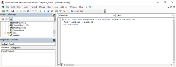
FIGURE 18-11: Writing your own function.

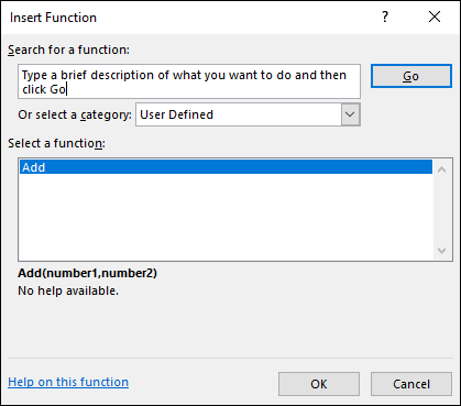
FIGURE 18-12: Finding the function in the User Defined category.

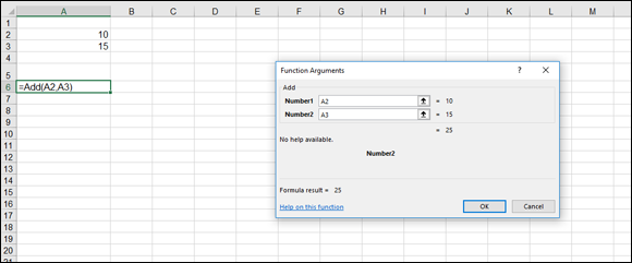
FIGURE 18-13: Using the custom Add function.

This is a very basic example of what you can do by writing your own function. The possibilities are endless, but of course, you need to know how to program VBA. I suggest reading Excel VBA Programming For Dummies, 5th Edition, by Michael Alexander (John Wiley & Sons, Inc.).

Macro-enabled workbooks have the file extension .xlsm.