8

THE AGRICULTURAL CHALLENGE IN THE TWENTY-FIRST CENTURY

ANNE O. KRUEGER

Patrick Messerlin has been a key contributor to understanding the costs of protectionist measures and the benefits of an integrated international economy. He has also been, in my judgment, exceptionally brave, taking on “sacred cows” at a time when the opinion of policymakers was firmly set in inappropriate directions and when the likelihood that opinion might change seemed small. I congratulate the organizers for recognizing Patrick, and Patrick for all that he has accomplished.

My focus is on world trade in agriculture. If some forecasts are right, the future problems of global agriculture will be associated with demand rising more rapidly than supply. Assuming those forecasts are right, the (relatively little) discipline over agriculture so far achieved under the World Trade Organization (WTO), and even that which would have been augmented under the Doha Round, is fighting the last war. WTO disciplines (including those proposed under Doha), while welcome, are based on the premise that there is a secular trend of falling world prices of agricultural commodities, and that distortions arise because of overproduction. If, instead, distortions start to take the form of export restrictions on the part of agricultural exporters, distortions may be quite different in the future, although protection by high-cost producers might still be part of the problem.¹

BACKGROUND

Although the liberalization of trade in manufactured goods was a triumph for the GATT/WTO over its first sixty years of life, the fate of trade in agricultural products was disappointing. Until the Uruguay Round, there was virtually no GATT/WTO discipline over trade in agricultural products. Many countries that were natural importers invoked “food security” as a basis for protection. Even some countries that should have had a comparative advantage in a number of agricultural commodities discriminated so much in favor of manufactures that they became importers!²

At the founding of the GATT after World War II, agricultural production was well below prewar levels in Europe and Japan, and it was natural that incentives would be given to restore productive capacity. And, in the case of the United States, because programs had begun during the Great Depression with the intention of protecting agriculture, it insisted on grandfathering these into the initial agreement. Meanwhile, many other countries invoked “food security” or “foreign exchange shortage” (especially in the case of developing countries) as a rationale for maintaining domestic prices well above world levels through import prohibitions, high tariffs, or quantitative restrictions on imports of agricultural commodities.

Agricultural production increased rapidly as disruptions from World War II were overcome. Although tariff barriers on manufactures were falling as a result of multilateral tariff negotiations, distortions resulting from protection for agricultural commodities and the search for food security increased the global misallocation of agricultural resources. Once agricultural production was above prewar levels in Europe, the Common Agricultural Policy (CAP) protected European farm prices and, for an extended period, resulted not only in increased protection but also in subsidization of exports for some agricultural commodities.³ The Japanese, and later the South Koreans, built high walls of protection against imports for many agricultural commodities, with tariff equivalents for rice and some meat products of several hundred percent.⁴

Although the United States maintained its program of price supports and other assistance for agriculture, it was a net exporter of agricultural commodities. If any one of the three groups—the Europeans, the Americans, or the East Asians—had removed their farm programs unilaterally, adjustment costs would have been far greater than if they could have found a coordinated approach. To a degree, each used the others’ protection as a rationale for maintaining its own. Agricultural protection was crying out for a multilateral solution.

Most developing countries, meanwhile, were attempting to provide incentives for increasing domestic production of manufactures, using tariffs and quantitative restrictions on their imports (on agricultural commodities, on consumer goods, and even on farm inputs), with overvalued exchange rates, which penalized agricultural exporters.⁵ There were also high prices for domestically produced manufactured inputs for agriculture and imported consumer goods for farmers and imports in many poor countries.

For the world as a whole, there appeared to be a secular trend toward falling relative prices of agricultural commodities, and the global problem, or “challenge” if you prefer, appeared to be to reduce distortions in agriculture primarily by reducing incentives for production in developed countries at above world prices. Yet, increasing agricultural productivity in some developing countries by enough to meet upward shifts in their demand from rising per capita income and growing populations appeared to be a virtually insurmountable challenge.

THE URUGUAY ROUND

Until the Uruguay Round, launched in 1986, it had proved impossible to agree on any multilateral discipline over production and trade in agricultural commodities. In part this was because of the domestic priorities individual countries and groups of countries gave to their farm objectives. But in part the problem was that, unlike manufactures, agriculture was protected by a large number of policy instruments, so even estimating the level of protection was challenging. Different countries adopted differing combinations of import tariffs and quantitative restrictions, domestic price and income supports, subsidized credits for farmers, and export subsidies to try and achieve their objectives. Moreover, again unlike for manufactures, there was widespread belief that developing countries as a group had a comparative advantage in production of agricultural commodities and were harmed by the “overproduction” in developed countries. Whereas industrial countries had collectively agreed to reduce tariffs on manufactures (in which they generally did have a comparative advantage) and could lead the negotiations, they were reluctant to alter their farm policies; and developing countries had, until Uruguay, been free riders on the tariff cuts (almost entirely on manufactures) negotiated among the industrial countries and did not consider taking leadership or even urging reducing agricultural protection.⁶

By the mid-1980s, technical research had suggested that the measure “producer subsidy equivalent” (PSE) could be used to render comparable the production levels in different countries despite their very different combinations of border and domestic measures to support agriculture.⁷ At about the same time, budgetary burdens, particularly in the European Union, led to pressure to modify farm support programs.⁸

The Uruguay Round achieved the first serious GATT/WTO discipline over agriculture, although there was disappointment that the ceilings negotiated in the round were not more binding.⁹ It was agreed that agricultural programs could be categorized in one of three pillars: a green box, into which policies toward agriculture that were judged to have virtually no (trade-distorting) effect on output of individual commodities were placed; a blue box for “moderately distorting” measures; and an “amber” box, which contains the trade-distorting measures.¹⁰

The green box was to contain policies such as land set-aside programs for environmental purposes, research and development support, and subsidies not linked to production levels. Only the amber box commodities were subject to ceilings, as it was thought that blue box measures would be a step toward reducing distortions.¹¹ Countries were to list in the amber box all the measures which increased incentives to produce individual commodities above those that would have existed at world prices.

However, the actual indicator to be employed to measure distortions was not the PSE, but rather the aggregate measure of support (AMS).¹² The AMS was to be calculated for each major commodity as the percentage of the various price-distorting measures (including tariffs, subsidies without ceilings on land use or production, and administered prices at above world levels) of the reference price. The reference price was the l986–1988 price, rather than the prevailing world price. Hence, in years when world prices were above those of the reference period, the AMS overstated the distortion, since the divergence between domestic prices and world prices was smaller than the AMS, while in years of low world prices, the AMS understated the distortions.

Countries were to notify the WTO of their measures annually, and the Committee on Agriculture was to meet regularly, evaluate whether policies were appropriately categorized, and estimate the resulting magnitudes. There were negotiated AMS targets for each country in the Uruguay Round. AMS included limits for major individual commodities (such as wheat) and overall totals (the total aggregate measure of support, or TAMS) over all commodities. The AMS and related measures were negotiated for each country and included in the Uruguay Round agreement.¹³ The Uruguay Round also required an average tariff cut of 36 percent, the conversion of import quotas into tariffs, and a number of other measures to reduce agricultural protection. All of these were, in principle, designed to reduce total protection to agriculture, primarily in industrial countries. But by the time the ceilings and categories were negotiated, the actual reductions were far less than the aggregate measures suggested.

POST–URUGUAY ROUND AGRICULTURAL SUPPORT TRENDS

Figures 8-1a through 8-1c provide an indication of what happened from l986 to 2018, both to the PSEs and the TAMS, for the EU, Japan, and the United States, respectively. The data are in the respective national currencies. Relative to the levels in the latter part of the 1990s, by both measures support has fallen. Part of this drop reflected higher world prices. But the divergence between the PSEs and the TAMS increased as countries shifted from direct price supports to other means of assisting agriculture. For Japan and the United States the value of the PSE and TAMS both fell substantially in the 1990s. The measures were as close together as they were because high world prices resulted in less support for farmers.

FIGURE 8-1A. European Union: Producer Subsidy Equivalents (PSEs) and Total Aggregate Measure of Support (TAMS), 1966–2017

Source: PSEs are from the OECD and AMS are from WTO.

FIGURE 8-1B. Japan: Producer Subsidy Equivalents (PSEs) and Aggregate Measure of Support (AMS)

Source: PSEs are from the OECD and AMS are from WTO.

FIGURE 8-1C.  United States: Producer Subsidy Equivalents (PSEs) and Aggregate Measure of Support (AMS)

Source: PSEs are from the OECD and AMS are from WTO.

There was, and is, considerable variation in PSEs among farm commodities and among countries. In the United States, for example, average PSEs (as a percentage of gross farm receipts) in 2002–2004 were 33 for rice, 57 for sugar, and 40 for milk, but 4 for poultry, pork, beef and veal, with an overall PSE of 18. Japan’s PSEs for rice, wheat and oilseeds were 83, 85, and 57, respectively, with an overall average of 56.¹⁴ PSEs do not include general support for agriculture, but only those measures that affect the incentives to produce particular crops. Thus the PSE does not include measures that provide price supports for a crop if they also restrict acreage so that production cannot be increased. When there is a food subsidy, such as in the US Food Stamp Program (now called SNAP [Supplemental Nutritional Assistance Program]), that does not count as part of the PSE but does count in the TAMS. Measures that are not commodity-specific include items such as water subsidies not tied to individual crops, research, and land set-asides for environmental reasons. To simplify exposition, the PSE is the metric reported in the remainder of this chapter because it is a better measure of distortions than the AMS.¹⁵

Figure 8-2 gives indicators of the magnitudes of the PSEs as a percentage of farm receipts since l986–1988 for the OECD member countries. For the OECD as a whole, the PSE fell from around 30 percent in the 1990s to below 20 percent after 2010. Declines are also observed for the United States, the European Union, and Japan. This drop primarily reflects two phenomena: a decline in applied import tariffs—by 6 percentage points since 2000 (OECD 2019) and a shift in support away from direct price supports (with no acreage limits) to other programs and price supports with acreage limits. It is by no means assured that PSEs would remain so low if world prices of agricultural goods were to fall. As noted previously, higher farm prices imply that PSEs will fall even without any government action. Overall agricultural prices have increased over the period, although with significant volatility. Between 2010 and 2014–2015, for example, many agricultural commodity prices fell substantially, before recovering in 2016–2017. At this writing in 2020, they stand around 20 percent below 2010–2013 levels.

FIGURE 8-2.  Producer Subsidy Equivalent (PSE) Indicators, 1986–2018

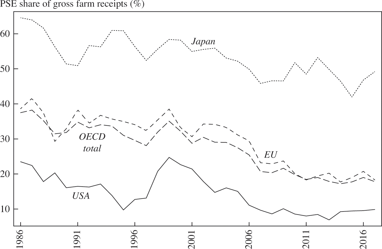
Source: OECD (2019).

Prices of agricultural commodities peaked in 2007–2008. As a result, in most countries farm incomes were at all-time highs: in the United States, the average farm family income had already risen above average urban family income by 2002, and rose further above it when farm prices peaked.¹⁶ Since then, PSEs as a share of gross farm receipts fell by 10 percentage points in the EU, the United States, and the OECD as a whole (figure 8-2). One reason for this is that, overall, in the period since the Doha Round was launched, average world food prices rose.

Farmers, however, experienced more of a roller coaster than the PSEs indicate. Farm prices fell during the Great Recession, then rose about 20 percent by 2011, and another 15 percent by 2015–2016. Thereafter, however, they fell, and the index stood at only 94 in 2019. As if that were not enough, the prices of farm inputs (e.g., feed, seed, and fertilizer), which had moved at about the same rate as prices received until 2014, began falling. The index, which stood at 115 in 2014 (on a 2011 base), fell to 93 in 2019 (OECD 2019). The pain of falling output prices was magnified by the continuing rise in input prices. Once the WTO had established the PSE limits, governments shifted some of their support from those covered in the PSEs to others. Consequently, while government payments to farmers rose, the PSEs changed very little.

US real farm income peaked in 2013 at $123.4 billion and fell to $63.1 billion in 2018.¹⁷ The most recent American farm bill, which is up for renewal about every five years, was passed in 2018.¹⁸ A major expenditure under the farm program, SNAP, was reduced from its earlier levels in the last two acts. Other than that, and shifting away from payments counted in PSE measures, the Farm Bill was not significantly changed in the two versions that passed after the Great Recession in 2014 and 2018. In Europe as well, PSEs were lower than they had been before the PSE limits, but were partially offset by policies outside the PSE restrictions.

For present purposes, two points are relevant. First and most important, the Uruguay Round established a framework for WTO discipline over support to agriculture. Second, the Uruguay framework was based on the assumption that the problem was that incentives for more production were greater than they would have been had commodity prices cleared in an efficient world market. Fortunately (or otherwise), prices of agricultural commodities rose sharply as the Uruguay Round constraints were gradually coming into effect (starting in 1995). The result was that many countries had to do little or nothing to meet their commitments under the round, since farm prices and incomes were generally sufficiently high that intervention costs were below the limits set forth in the final agreement.

When countries needed to act to meet their Uruguay Round constraints, there was some reduction in support, but in many cases there was a shift away from supports for commodity prices (and acreage under production) to direct income support. The OECD estimates, for example, that Switzerland’s PSE for farmers fell from 77 percent of its total support to 55 percent, while its total support fell from over 90 percent to around 70 percent in the fifteen years following the Uruguay Round. But the most salient facts are that discipline had begun, and that countries were largely in compliance with it.¹⁹

When world prices of agricultural commodities fell early in the 2000s, most countries’ programs were within the limits set under the Uruguay Round—both because of the 1986–1988 base and because countries had shifted from reliance on direct price supports to income supports with acreage limitations or other exemptions. Farm incomes were therefore effectively protected at the same time that the limits on distortive measures negotiated in the Uruguay Round were observed. Nonetheless, there could not be any question but that industrial countries were still subsidizing their farmers heavily. For the OECD as a whole, PSEs as a percentage of gross farm receipts were 40 percent in l986 and around 30 percent in 2001 when the Doha Round was launched. For the European Union, the corresponding figures were 45 percent and 35 percent, while those for the United States were 25 percent.

THE DOHA ROUND

The Uruguay Round ceilings are, of course, still in effect, as there has been no closure to the Doha Round. During the initial years of Doha negotiations, strengthened disciplines were negotiated and tentatively agreed on for agriculture. If these measures had become part of a final Doha Round agreement, they would have further constrained distortive agricultural policies.²⁰ As Orden, Josling, and Blandford (2011b, 420) concluded: “a Doha agreement built on the December 2008 draft modalities would achieve real progress on the path toward substantial progressive reductions envisioned in the 1994 Agreement on Agriculture. A Doha agreement … would impose some meaningful constraints, especially for developed countries.”

There can be little doubt that acceptance of these measures would improve the efficiency of world agriculture. Whatever the secular trend in world prices of agricultural commodities, there are bound to be periods of low prices, and constraints on the degree to which there can be incentives for additional production would serve to reduce the variance in world prices of agricultural commodities. Thus, an upward secular trend could reverse at a future date, just as the secular downward trend of much of the past fifty years has perhaps now been reversed. Hence the ceilings negotiated in Doha would represent progress.

This would be especially true if meaningful bounds on support for commodities such as ethanol and cotton could be included in the agreement. Despite the progress that would be represented should the 2008 undertakings be enacted, there are special problems with a few key commodities, and those result in considerable distortions in the global economy.

Perhaps the most serious from a global viewpoint is ethanol—it is estimated that 17 percent of the global maize crop is now destined for production of biofuels (OECD/FAO 2019). Originally mandated by the US Congress as an environmental measure consistent with renewable energy resources, the Renewable Fuel Standard (RFS) was established by the Energy Policy Act of 2005 and expanded in 2007. The RFS requires that transportation fuels contain an increasing volume of renewable fuels over time. The mandate was 4 billion gallons of renewable fuel in 2006. As of 2019, the Environmental Protection Agency (EPA) had increased the mandate to 19.9 billion gallons (Bracmort 2019).²¹ One result of the mandate, together with subsidies for maize production—totaling roughly $90 billion between 1995 and 2010 (not including ethanol subsidies and the mandates) (Foley 2013)—is that the United States has become the leading global producer of ethanol, accounting for 50 percent of world output, and the second largest producer of biodiesel (19 percent of world output) (OECD/FAO 2018).

The environmental impact of the RFS is questionable. The advanced biofuel component of the RFS, which would yield greater greenhouse gas emission reductions and generate fuel from nonfood biomass, has missed the statutory targets by a large margin. The initially assumed environmental benefits of ethanol from maize production are small at best because of the energy, fertilizer, and other inputs used in growing corn and in ethanol production (Foley 2013). If the mandated increases in the ethanol content of gasoline were not adjusted by the EPA, much of the US maize crop would have to go to ethanol. As it stands, about 40 percent of the US maize crop is used for biofuel production,²² and sizable acreage has been diverted from soybeans and other crops or been brought into production. The sharp upward shift in demand for corn for ethanol is estimated to have accounted for 25 percent or more of the increase in world grain prices in the late 2000s. Reducing the use of corn for fuel would reduce upward price pressures, lower demand for scarce natural resource inputs, including land, and expand food output.

The magnitude of subsidies for ethanol production in the United States has been reduced since Congress removed a 54 cents per gallon specific tariff on imports of ethanol, as well as tax credits to refiners of 46 cents per gallon in 2011. The increased requirements for ethanol production were deemed sufficient protection, and there was little protest from the industry. Redressing the ethanol situation will be difficult (since large investments have been made in ethanol plants), but it will become even more so as time passes. The impact on food supply and prices and the lack of benefits makes a clear case for removal of support policies for ethanol, but the refiners and corn growers are strongly resistant.

Another high-cost program is the US cotton price support program. It was expanded markedly in the late l990s and resulted in a large increase in US production, much of which was exported. The result was a sharp drop in world cotton prices, with pronounced impacts on some small countries for whom cotton was the major export and a large part of small farmers’ incomes. West African cotton-exporting countries were especially hard hit because many small farmers relied on cotton for most, or even all, of their income. The four African exporters consider that a sharp change in the cotton program, or compensation for their reduced export prices, is essential for them. Brazil pursued a WTO dispute case and eventually won some compensation. Negotiating a significantly lower cap on the PSE for cotton would result in a higher world price for cotton, with benefits for efficient use of agricultural resources and for the exporting countries.²³

LOOKING TO THE FUTURE

Completion of the Doha Round, including the elements of what emerged in 2008 to strengthen agricultural disciplines, would have represented a significant step toward more efficient world agriculture. Even if it had been completed, much would be left for future negotiations. The EU, Japan, and the United States continue to have costly and inefficient farm support programs. Moreover, PSEs have been increasing in emerging economies, roughly doubling, from 5 to 10 percent, in the past decade.

As already seen, the disciplines negotiated in the Doha Round would have further constrained countries’ use of distortive measures in years of falling prices. But while the Doha Round has languished, it is quite possible that the distortions in world agricultural production may be changing. During the period of peak prices in 2007–2008, a number of exporting countries (including, in particular, Argentina, Russia, and Ukraine) imposed quantitative restrictions or outright prohibition on the export of key commodities. Table 8-1 lists some of the export restrictions applied to agricultural commodities over the ten quarters starting from the end of 2008. The list is almost certainly not comprehensive and only includes measures that were listed in sources accessible to Global Trade Alert compilers. The motive for imposition of restrictions was to keep domestic prices below world prices.

TABLE 8-1. Partial List of Restrictions on Agricultural Exports, 2008–2011

Country		Restriction		Date imposed
India		Cap on cotton exports		August 16, 2011
India		Extension of ban on edible oil exports		August 16, 2011
India		Partial removal of export duty on basmati rice		July 4, 2011
Kyrgyz Rep.		Temporary export taxes on agricultural products		July 1, 2011
Serbia		Temporary export restrictions on wheat and flour		April 1, 2011
Moldova		Export ban on wheat		February 2, 2011
Ethiopia		Ban on export of raw cotton		November 15, 2010
Ukraine		Export quotas on agricultural products		October 4, 2010
India		Extension on ban of pulses exports		August 19, 2010
India		Ban on cotton exports replaced by licensing		May 21, 2010
Argentina		Reference prices for designated exports		March 5, 2010
Argentina		Export registration requirements		November 1, 2009
Indonesia		Export tax on cacao beans		April 1, 2010
Argentina		De facto ban on bovine meat exports		February 1, 2020
Kazakhstan		Temporary ban on rice and milk exports		December 1, 2008
Egypt		Repeat ban on rice exports		September 24, 2010
Source: Simon Evenett, provided through correspondence from the Global Trade Alert database, November 2011.

Under present arrangements, such measures do not violate WTO disciplines. While there are limits on distortive border and domestic measures that encourage agricultural production, there are no constraints on export prohibitions or restrictions.²⁴ But there are many forecasts of shortages and hence rising prices of agricultural commodities over the next half century, with rising populations and real income growth. If that is correct (and it seems to be the view of the majority of agricultural economists and the agricultural policy community), the danger of increased distortions to agricultural production almost certainly arises more from the risks of export limitations and the reactions that they are likely to evoke. Not only will world prices rise further at times when export restrictions or prohibitions are imposed, but countries importing agricultural commodities will become concerned about their long-term food security and resort to protective measures to induce more domestic production.

The agricultural agreements already negotiated in Doha are desirable not only because the future trajectory of supply and demand is not certain, but also because even if the past trend toward lower prices is reversed, there are bound to be price fluctuations and therefore periods of low prices—as well as periods of high prices.

To increase the efficiency of world agriculture and to prevent (or restrict) the emergence of a new set of distortive policies guarding against high prices rather than low ones, discipline over export restrictions is also needed.

It is easy to see the dangers. Export restrictions or prohibitions on the part of countries with a comparative advantage would not only distort world agriculture, but would also intensify any trend toward higher prices for agricultural commodities. If exporters impose restrictions during periods of high prices, it is very likely that importing countries will respond at least partially by increasing protection for their own domestic agriculture. This might be done in retaliation, or in the name of food security. And, if prices of agricultural commodities are expected to continue to increase (or even to be maintained at very high levels), policymakers in importing countries could also argue that higher domestic production would be, or would shortly become, economic.²⁵ If that were to happen, distortions in world agriculture would increase. Moreover, it is likely that the average prices of farm commodities would rise even more than they would with an efficient allocation of resources, while the fluctuations in world prices of agricultural commodities would intensify (as, perhaps, would fluctuations in individual countries as exporters lost their markets and importers were increasingly affected by domestic supply variations).

FIGURE 8-3.  Top Five Users of Agricultural Export Restrictions, 2009–2018

Source: Global Trade Alert.

Since 2010–2012, the use of export restrictions fell as world prices dropped (figure 8-3). There is no assurance, however, that a similar pattern in the use of export restrictions will not reemerge if prices spike again. Several countries imposed restrictions on exports of certain agricultural products in the first half of 2020 in the context of the COVID-19 pandemic. Although the use of such measures was relatively limited compared to 2007–08 (a total of thirty-two countries imposed forty-nine export restrictions between January and July 2020, and many of these were rescinded during this period), it illustrated again the willingness of countries to impose export restrictions.²⁶ If some countries that normally export impose quantitative restrictions or prohibitions on exports of key commodities at times of high prices or in response to supply shocks, the fluctuations in world prices of agricultural commodities would intensify. World prices of traded agricultural commodities whose exports are restricted will rise more during periods of high prices than they otherwise would. That, in turn, would almost certainly induce reactions from countries that, in an efficient allocation of resources, would be net importers of agricultural commodities.

Domestic prices in “natural” exporters would be lower because of restrictions on exports, and hence there would be less production and more consumption, and smaller exports. Moreover, farmers in “natural” exporting countries would experience lower prices, and therefore incomes, both in times of high prices (because domestic prices would be below world prices) and in times of low prices (because the “natural” importers would be producing more but consuming less because of higher prices, and thus importing less). Hence, at a time of increasing upward pressure on prices of agricultural commodities (as is assumed here), production would shift from former exporters (the lower-cost producers) to former importers (the higher-cost producers). If, as is believed, it is desirable to increase agricultural output efficiently, the net effect would be in exactly the opposite direction. One of the few achievements of the Doha Round was a 2015 agreement to ban agricultural export subsidies. Complementing this with an equivalent agreement to ban export restrictions would be very desirable.

CONCLUSION

Completion of the Doha Round would improve the world agricultural economy. It would, nonetheless, leave numerous challenges. High on the list is the difficulty that will arise if the trend for world agricultural prices over the past half century is reversed and a secular upward trend replaces it. Although the future trajectory of agricultural prices cannot be forecast with certainty, most careful assessments project increases. If prices rise, the Uruguay Round disciplines over agriculture and their intensification under it would still be useful, but the WTO will be lacking disciplines over the additional distortions that might arise in times of rising prices. For that purpose, an agreement to refrain from export restraints when prices rise would be needed.

Such an agreement would benefit agricultural exporting countries and would result in lower average world prices than would be the case if exporters (importers) move toward export restrictions (higher levels of protection against imports). If the world’s problem is, as would seem likely, rising world prices, there is a strong reason for bringing export restrictions under discipline now before future runups in prices induce more such measures. If the future holds higher prices for agricultural commodities, it will also be highly desirable to find disciplines that balance trade-offs between environmental concerns and the supply of agricultural products much more effectively than has happened to date. This could take the form of a discipline, such as that governing phytosanitary concerns, that requires scientific evidence of the supposed benefits of environmental measures and use of the least-cost way of achieving the desired environmental outcome.

The prospect that some distortions in world agriculture could be removed through two large preferential trading arrangements, the Trans-Pacific Partnership (TPP) and the Transatlantic Trade and Investment Partnership (TTIP), has not materialized. The former did constrain some highly protectionist countries, including Japan and South Korea. Thus the Comprehensive and Progressive Agreement for Trans-Pacific Partnership (CPTPP), the successor to the TPP which was rejected by the Trump Administration, will entail a reduction in agricultural protection in East Asia. But it will not do so in the United States since the United States withdrew from the TPP and put the TTIP negotiations with the EU on hold. Even if agreements spanning the EU and United States were concluded, it seems evident that some of the distortions to agriculture (such as ethanol and cotton) would probably not be greatly reduced, as too many producers of cotton (in Africa especially) and producers and consumers of maize are not part of the negotiations. The need for global disciplines remains.

A major change in the global agricultural economy came about in 2018 when the United States initiated its trade war with China. The United States imposed tariffs on a number of Chinese goods, and the Chinese retaliated in part by purchasing soybeans, corn, and other grains from other suppliers. Part of the recorded drop in US farm prices in 2018 and early 2019 was attributable to the shift in those Chinese purchases from the United States to Brazil and other countries. Although the US administration committed $28 billion to US farmers, there were important political protests against the resulting decline in farm prices. As of mid-2020, many of the American tariffs and the measures the Chinese took in response are still in place and it remains to be seen if the January 2020 agreement between the United States and China, under which China undertook to boost imports of American agricultural products, will be implemented. The outlook for tariff removal is not clear.²⁷

It would clearly be desirable to revive multilateral efforts to bolster disciplines on agricultural policies. Even if all that is feasible is what was on the table in 2008, there would be gains. For agriculture, increased discipline would benefit the global economy. The opportunity cost of not completing the Doha Round is not only that existing disciplines on domestic support have not been tightened. Issues of equal importance, such as the need for discipline over agriculture in times of high prices, require urgent attention.

NOTES

After I wrote a first draft of this chapter early in this decade for the conference in honor of Patrick Messerlin, farm prices rose and then began falling again after 2014–2015. Little has changed by way of policy. I am more heavily indebted to David Orden, Lars Brink, and Tim Josling than is usually the case with an acknowledgment. They provided support not only by providing data but also in navigating the complexities of the Uruguay Round. I am also grateful to Simon Evenett for sharing his Global Trade Alert (GTA) results, to Matteo Fiorini for updating the GTA and agricultural support data through 2018, and to Farouq Ghandour for research assistance. The responsibility for any errors of fact or interpretation in the chapter is solely mine.

1. 1. Challenges that may arise for global efficiency of agricultural production because of future environmental considerations are not dealt with in this chapter. A brief discussion of the impact ethanol subsidization has had on agricultural production and food prices is provided to give an illustration of the sorts of problems that might arise.

2. 2. See Krueger (1992) for estimates for some countries in the mid-1980s.

3. 3. It will be recalled that the variable levy under the CAP maintained high prices for producers and in some years resulted in production in excess of domestic consumption, resulting in exports that were subsidized.

4. 4. See Anderson and Hayami (1986) for a discussion.

5. 5. Nominal exchange rates were kept fixed for long periods despite inflation rates much above those in the developed countries, and hence overvaluation was rife. The rationale for this was that it would make imported capital goods cheap and thus enable more investment. The difficulty was that, with overvalued exchange rates the incentives for exports were weakened, foreign exchange earnings rose less rapidly than demand for foreign exchange, or even stagnated, and hence exchange controls tightened and imports of capital goods could not increase as had been expected.

6. 6. It is not entirely clear that all developing countries have identical interests in agriculture. Some are net importers of food products, and others are net exporters; some have comparative advantage in tropical commodities, and some in temperate. But it was considered that developing countries as a group had an interest in reducing high levels of protection for agriculture in advanced countries.

7. 7. The acronym PSE is used to denote both “producer subsidy equivalent” and “producer support estimate.”

8. 8. By that time, the European Union historically had difficulties with mounting inventories of supported agricultural commodities. Perhaps the support program that most vividly typified the problem was that for butter. The “butter mountain” became a standard jibe at the CAP. But the variable levy (which took import proceeds and distributed them to farmers for “double protection” and the export subsidies of the CAP) led to widespread pressure for program modification.

9. 9. The aggregate measure of support, the metric actually used by the WTO, is somewhat different than the PSE proposed by the OECD. See later discussion of the differences between the two measures.

10. 10. The volume from Orden, Josling, and Blandford (2011b) is invaluable in analyzing the agricultural provisions of the outcome of the Uruguay Round.

11. 11. This meant, however, that Japan, for example, could reduce its reported AMS by maintaining high levels of border protection for rice, while eliminating its administered price which had been well above world levels.

12. 12. Orden, Josling, and Blandford (2011b), especially the chapter by Brink (2011), provide extensive discussion.

13. 13. See Brink (2011) for a detailed exposition.

14. 14. Estimates are from Elliott (2006, 29, table 2.4).

15. 15. Even PSEs suffer from the property that the same legislated farm support program can result in differing levels of distortion in different years depending on world prices and the type of protection accorded in domestic programs. A guaranteed minimum price, for example, would confer no protection (or distortion according to the PSE measure) in a year when world prices were above the guaranteed minimum. Such a guarantee, however, could nonetheless influence incentives for producing the crop by reducing uncertainty.

16. 16. It is estimated that a typical farmer in US corn-producing states was earning between $750,000 and $1.4 million annually by 2011 (Mufson 2011).

17. 17. USDA forecast and numbers as reported in US Department of Agriculture, NASS highlights, on July 1, 2019, at www.nass.usda.gov.

18. 18. The interested reader can learn more in the volume by Smith, Glauber, and Goodwin (2018).

19. 19. From appendix tables in OECD (2009).

20. 20. See appendix B of Orden, Josling, and Blandford (2011a) for an abridged text of the agreement.

21. 21. The statutory goal to be achieved in 2022 is 36 billion gallons, a target that will not be achieved (Bracmort 2019). No more than 15 billion of the 36 billion gallons may be corn-based.

22. 22. See data from the Alternative Fuels Data Center at https://afdc.energy.gov/data/10339 and the US Department of Agriculture at https://www.ers.usda.gov/data-products/us-bioenergy-statistics/us-bioenergy-statistics/#Supply%20and%20Disappearance.

23. 23. Glauber (2018) discusses changes in US cotton support policy and advocates shifting away from the changes imposed in the 2014 Farm Bill that removed direct and countercyclical payments.

24. 24. Of course, under Doha, subsidization of agricultural exports was to cease, but that again is a measure protecting against glut.

25. 25. Martin and Anderson (2012) have estimated that, in the 2006–2008 agricultural price surge, 45 percent of the increase in the price of rice and 30 percent of the change in the price of wheat can be explained by changes in border protection rates. Many importers had lowered their border protection as export restraints were imposed elsewhere (in response to rising prices) to ease the upward pressure on domestic prices, which exacerbated the impact on world prices of export restrictions.

26. 26. See EUI, Global Trade Alert and World Bank, Tracking Pandemic-Era Trade Policies in Food and Medical Products, https://www.globaltradealert.org/reports/54.

27. 27. The “phase 1” deal concluded by China and the United States in January 2020 retained the 25 percent tariffs imposed on $250 billion of Chinese exports but cut US tariffs on an additional $120 billion of Chinese exports imposed in September 2019 by 50 percent, to 7.5 percent, and suspended the US threat to impose punitive tariffs on those exports not already targeted by the United States. The main feature of the agreement was a promise by China to increase imports from the United States within two years by $200 billion more than the country had imported in 2017. See “Economic and Trade Agreement between the Government of the United States and the Government of the People’s Republic of China, January 15, 2020,” https://ustr.gov/sites/default/files/files/agreements/phase%20one%20agreement/Economic_And_Trade_Agreement_Between_The_United_States_And_China_Text.pdf.

REFERENCES

• Anderson, Kym, and Yujiro Hayami. 1986. The Political Economy of Agricultural Protection: East Asia in International Perspective. Sydney: Allen and Unwin.
• Bracmort, Kelsi. 2019. “The Renewable Fuel Standard (RFS): An Overview.” Congressional Research Service R43325. January 23.
• Brink, Lars. 2011. “The WTO Disciplines on Domestic Support.” In WTO Disciplines on Agricultural Support: Seeking a Fair Basis for Trade, edited by David Orden, Timothy Josling, and David Blandford, 23–58. Cambridge University Press.
• Elliott, Kimberley Ann. 2006. Delivering on Doha. Washington, D.C.: Center for Global Development.
• Foley, Jonathan. 2013. “It’s Time to Rethink America’s Corn System.” Scientific American, March 5.
• Glauber, Joseph. 2018. “Unraveling Reforms? Cotton in the 2018 Farm Bill.” Washington, D.C.: American Enterprise Institute, January.
• Krueger, Anne O. 1992. The Political Economy of Agricultural Pricing Policy: A Synthesis of the Political Economy in Developing Countries. Johns Hopkins University Press.
• Martin, Will, and Kym Anderson. 2012. “Export Restrictions and Price Insulation during Commodity Price Booms.” American Journal of Agricultural Economics 94 (2): 422–27.
• Mufson, Steven. 2011. “Ethanol Subsidy Fight Not Over.” New York Times, June 16.
• Orden, David, Timothy Josling and David Blandford. 2011a. “The Difficult Task of Disciplining Domestic Support,” in David Orden, Timothy Josling and David Blandford (eds.). WTO Disciplines on Agricultural Support: Seeking a Fair Basis for Trade. Cambridge University Press, pp. 391–432.
• ________, eds. 2011b. WTO Disciplines on Agricultural Support: Seeking a Fair Basis for Trade. Cambridge University Press.
• Organization for Economic Cooperation and Development (OECD). 2009. Agricultural Policies in OECD Countries: Monitoring and Evaluation. Paris.
• ________. 2019. Agricultural Policy Monitoring and Evaluation 2019. Paris.
• OECD/Food and Agriculture Organization of the United Nations. 2019. “Biofuels.” In OECD-FAO Agricultural Outlook 2019–2028. Paris: OECD Publishing.
• Smith, Vincent H., Joseph W. Glauber, and Barry K. Goodwin. 2018. Agricultural Policy in Disarray. Washington, D.C.: American Enterprise Institute.