Lesson 2 – Basic File Operations & Setting up Excel the Way You Want It

In Lesson 1 you were introduced to several key elements about both spreadsheets and Excel in general:

• • What is a spreadsheet?
• • What Excel is and the role it plays in the world of spreadsheet applications.
• • Some of the terminology specific to working with both spreadsheets in general and Excel itself.
• • What you can do with Excel in personal, business, and academic applications.
• • Understanding the Ribbon Interface
• • Developer Tab – We discussed how Microsoft gives you the ability to access the Visual Basic for Applications programming language to automate repetitive tasks, and do things that you just couldn’t do otherwise (like automate e-mailing a workbook with a push of a button).
• • Workbook & Worksheet navigation, including some keyboard shortcuts
• • Getting help from the resources that Microsoft has made available both within and outside of Excel

In Lesson 2 we’ll dive deeper into Excel itself and teach you how to get around the Ribbon interface by exploring all of its various elements and showing you what each one does. Again, this isn’t going to teach you how to use each one of their various elements, but it will serve as an introduction, so that when you start to get more comfortable with Excel you’ll have the knowledge to know where to look for key elements. This lesson will primarily focus on the File tab (Office Button in Office 2007), and show you how to customize Excel to meet your personal needs each time you open it. There is a lot of detail in this lesson, as it also focuses on some of the important aspects of file/document management (which will apply to any Office application), how to save files, when and where. If you’re relatively comfortable with the Office environment, then you’ll breeze through a lot of it.

 

Figure 16  

The File Tab

When you first open Excel, Microsoft has set your default options (preferences) to give you the most standard and user friendly options it can. If you’re somewhat familiar with Excel there are certain things you might want to change, because hey, what’s right for the “default” user may just not be right for you. And even if you’re not all that familiar with Excel there will probably be some things you‘ll want to change. Fortunately, Microsoft understands this, and they let you change it. Before we discuss how to change the Default Options, we go over what each item in the File tab represents, although for the most part they’re relatively straightforward:

To get started, we’ll click on the File tab (in Office 2007 this would be the Office button) and you’ll see the following options:

Save – This Saves the active workbook. It’s fairly simple, but often forgotten until it’s too late! Regularly saving your work is paramount! But make sure that if you open a workbook and make changes to it you’re absolutely sure you want to keep those changes before you Save the workbook! Otherwise your previous work will be overwritten by the new, and your chances of recovery are slim! (Unless you have a backup version you can recover). Untold work around the world gets lost because of this every day (this stands true for any application)! Just remember, Save First, Save Often!

Save As – This will let you save the active workbook as something else. Let’s say you make some changes to a workbook and you want to keep them, but not alter the original workbook, you would use the Save As option. When you Save As you’ll be presented with an application dialog box like this:

 

Figure 17  

• • The Save As dialog will take you directly to the Folder in which the active workbook was opened. Notice that the File Name is highlighted, allowing you to immediately enter a different name. If you don’t do that and try to Save Excel will ask you about it:

 

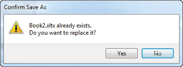
Figure 18  

• • If you hit Yes, you WILL save over whatever was in your workbook before you made any changes! If you don’t want to do this, then just hit No and you’ll still have the chance to enter a new workbook name.
• • From here you can choose a different workbook name, and browse to the location of your choice. Again, one of the first things you should do when making changes to an existing workbook is perform a Save As if you want to keep the original work! Otherwise you stand a very good chance of losing it! This becomes especially important when you start working on complex models that you want to keep intact (they don’t even have to be complex actually; lose an hour’s worth of work and you’ll be upset). To reiterate: untold hours of work get lost and have to be recreated daily around the world because of this.
• • The Save As dialog gives you some additional options that can be important with regards to who you might be sharing your workbooks with later, but you first need to be aware of some naming conventions when you try to save a workbook. Microsoft has done a great job of expanding the rules for file names, but there are still some limitations (and if you break them you’ll find out when you hit the Save button and you’re rewarded with a wonderfully ambiguous error message):

 

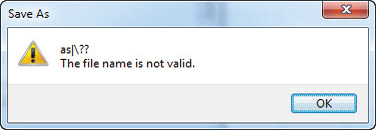
Figure 19  

• • Suffice it to say, you can’t use the following characters in an Excel filename (or any other Windows file name for that matter): *|\?:”<>?
• • Next on the list with the Save As dialog is the file type you can select. You’ll see the drop-down selections directly beneath the File Name dialog. This will let you save your workbook in any manner of ways. In general the default option is fine, but you do need to know about the differences, especially if you want to share a workbook with users who have earlier versions, or if you recorded some macros and want to keep them. All software applications have what’s called a file extension that’s appended to the end of the file name (e.g. “MyFile.doc”), which identifies it, and helps separate each application from the other. Where earlier versions of Excel only had two file extensions, Excel 2007/2010 introduced some new file extensions. Microsoft also gave you a lot of new ways to save your workbook with the new versions, fortunately you shouldn’t need to worry about anything but the default for now, which is an Excel Workbook (.xlsx). If at some point you do decide to start recording macros be aware that when you try to save a workbook with macros, Excel will prompt you to change the file type to a Macro-Enabled workbook. If you choose not to do so Excel will delete your macros!

 

Figure 20  

• • You also have more options in the Save As dialog than just saving:

 

Figure 21  

• • Display Options –This is where you set the way in which you want to see documents display in your Open, Save and Search dialogs. Some people prefer icons, especially if they deal with a lot of graphic images, while others prefer just a plain list of files. Details is the view you’ll see in all of the lesson examples. Detail shows the file name, Date modified, type and document size and will give you the most detail about the files you want to open or save.

 

Figure 22  

• • Author – This is the name that you entered into Office when you installed it. But you can click on the blue text to change it right here. You can also change it in the document properties, which we’ll get to shortly.
• • Tags – This is a short description of what’s in your workbook (e.g. Payroll, Schedule, etc.) This is supposed to help you speed up indexed searching when you use Windows Explorer to find files on your PC or network.
• • Title – Very similar to Tags, this is an extended description of your workbook’s function beyond the file name. Frankly, unless you’re dealing with thousands of documents, or saving and sharing files on a large corporate network neither Tags nor Titles will come in very handy for the everyday Office user.
• • Thumbnail – Clicking this will add a graphic image of your workbook that you can see when you search and open files. It’s generally a waste of resources since Excel has to save that image along with other file properties.
• • Tools – This option gives you some advanced settings that can come in handy if you need to have secure documents. There are four options here, but the one we’ll discuss is General Options as the others are more broad Windows options:

 

Figure 23  

Always create backup – This will create a backup copy of your workbook whenever you close it. This is a good idea if you don’t consistently back up files to an external source, but bear in mind that the backup copy will be created in the same folder as your workbook. Unfortunately, this means that if you lose access to the workbook’s location for whatever reason (hard drive failure, folder deletion, etc.) you’ll also lose the backup. Also note that a backup copy will be created as soon as you save your workbook, so if you accidentally save over a file, the backup will be a copy of what you saved over too.

 

• • Password to open – this is handy if you keep workbooks on a shared drive and you don’t want other people to access them.
• • Password to modify – This will allow people to open your workbook, but will require them to provide a password to make changes. It’s handy if you want to share your workbook, but don’t want others to make changes.
• • Read-only recommended – This option can be used on its own or in conjunction with the Password options. It gives you is the ability to save your workbook as a Read-only document. This means that others can access the workbook, but any changes they make can’t be saved unless they save the workbook as something else. Again, it comes in handy if you want to distribute your workbook, but don’t want people changing your original.

Open – This will call the Open dialog (by default it will open to whatever location you have told Excel to save to in the application Options, which we’ll cover shortly):

 

Figure 24  

• • Note the File Type balloon here. Similar to your Save As options, you have multiple options regarding the file types you can open, but the default is “All Excel Files”, so if you’re expecting to see a Text file show up here you won’t unless you chose a different option from the drop-down. Additionally, the file type options listed below “All Excel Files” are the document types that Excel can possibly open (in general, but it’s not always a given).

 

Figure 25  

• • If you select the All Files option and try to open an unsupported document type, like a Word document, Excel will try to do it, but you’ll either get a Wizard like this:

 

Figure 26  

• • Or garbage like this:

 

Figure 27  

• • That’s really not Excel’s fault, in fact it did the best it could to read what you wanted to open. You should know this because if you don’t you’ll be scratching your head for a bit until you realize you just tried to open a Word document in Excel (and it happens more than you might think!) If this does happen, just close the workbook and start over. You won’t cause any damage to the file you opened (unless you try to mess with the garbage you see above and resave it as the original document, then you will have some issues, so please don’t do that!)

 

Close - This will close the workbook. If you haven’t made any changes to the workbook since you opened it then it will close without any prompts. If you have made changes to the workbook then you’ll be asked if you want to save it before closing it. Sometimes you might want to open a workbook to make some quick assumptions, but close without saving them, so make sure not to confirm saving the workbook if that’s the case.

Info - This will open a new pane on the right side of the menu that displays all of the relevant workbook information:

 

Figure 28  

The information for a new workbook that hasn’t been saved will be dramatically different than one that has been:

 

Figure 29  

• • Compatibility Mode – This dialog will be here if the workbook has been saved as an earlier version of Excel. It lets you know that some features available in Excel 2007/2010 have been deprecated in order to make the workbook compatible with earlier versions.
• • Permissions – This dialog lets you know if the workbook has been protected. Selecting it will give you multiple options for distribution and protecting the workbook:

 

Figure 30  

• • Check for Issues – This dialog lets you evaluate the workbook for any potential problems before you share it. You’ll probably rarely ever find a need to use this feature.

 

Figure 31  

• • Manage Versions – This will let you know if there are any pre-existing versions of the workbook. Again, it’s not likely you’ll ever use this feature.
• • Thumbnail – This displays a thumbnail image of the active worksheet.
• • Properties – At the bottom of the Info pane there is an option to Show All Properties or Show Fewer Properties. You can manually edit any of the editable workbook Properties simply by left-clicking on them, making your change and clicking Enter. You can’t change intrinsic document properties like the Size, Modified/Created dates, etc.
• • Recent – The Recent files list will show you a list of your most recent activity:

 

Figure 32  

Note the little Pushpin icon, which will let you pin a file to the list so that it always appears at the top, no matter how long it’s been since you last opened it. In this example the workbook at the top has been pinned in place.

New – This will launch a dialog that gives you options as to what kind of workbook you want to create. You can choose from a blank workbook, sample templates that are stored on your computer, your personal templates, or browse from Microsoft’s excellent selection of templates online.

 

Figure 33  

 

Print – This will bring up a dual-screen dialog: your options for printing both the active worksheet and the entire workbook are on the left next to the File menu, while a preview of the active worksheet is on the right. There is a lot of detail behind this dialog, to the point that all of Lesson 7 is devoted to Printing and Page Setup, so we’re not going to spend any time on it here.

 

Figure 34  

Save & Send – This dialog was brand new in Excel 2007 and it represents some significant advancements with regards to distributing your workbooks.

 

• • Send Using E-Mail – This dialog gives you the option to send in various ways:
• • Send as an attachment – This will use your installed e-mail client. If you have Office that’s most likely going to be Outlook. This will not send through an Internet e-mail client like Gmail unless you have Outlook configured to manage your account.
• • Send a link – This will create a link to the workbook’s location in an e-mail, but the workbook needs to be saved in a shared location, like a document sharing site.
• • Send as PDF – Excel now supports native PDF creation, so you no longer have to have a PDF writer like Adobe Acrobat installed on your computer.
• • Send as XPS – This is a format that allows documents to be viewed online and retain its source formatting. Unless you plan on putting a lot of workbooks on the Internet, the odds of ever using this option are slim.
• • Send as Internet Fax – This feature allows you to send a fax directly from your computer, but it does require you to have an Internet fax service. Unless you deal with a lot of documents requiring physical signatures the E-Mail option will most likely be the one you use the most.
• • Save to Web – This is one of the best features to come along in quite some time. It allows you to save files directly to a Microsoft SkyDrive folder.

 

Figure 35  

 

Save to SharePoint – SharePoint is Microsoft’s corporate collaboration server. It’s used by most Fortune 1000 companies. But it’s incredibly expensive, which is one of the reasons that Microsoft launched the SkyDrive service, which is a perfect alternative for small businesses.

 

Figure 36  

• • Help – This dialog is a bit of a twist on the standard Helpfile dialog you’ll find in an Excel workbook. It does give you the option to access the standard Helpfile (although it would be silly to come all the way here just to get to that!). It primarily gives you access to the tools you need if you want to check if there are updates available for Excel, find your product key, or even if you want to see how to get a hold of Microsoft for support.
• • Add-Ins – This will list any available Add-Ins that have document preparation capabilities. In this example you’ll see Adobe PDF functionality. Because this functionality is already exposed in other places, it’s unlikely you’ll ever this menu this unless you’re in a specialized field that has an industry specific Add-In.

 

Figure 37  

Changing Excel’s Default Settings so They’re Right for You

Options – Finally, we’re getting to how you set up your defaults in Excel so that it does what you want. Some of the defaults you won’t bother changing from Microsoft’s factory settings, some of them you’ll only change this one time, and some you’ll change between workbooks depending on what you’re doing. Note that changing certain options will require you to Exit and restart Excel in order for them to take effect, but Excel will let you know. The Options menu has 10 individual sections:

• • General

 

Figure 38  

• • Show Mini Toolbar – This is a pretty cool feature that appears if you hover over a Ribbon control:

 

Figure 39  

• • Enable Live Preview – This is something Microsoft has been working on for a while, and it’s pretty slick. Essentially, it allows you to preview the effects of a change to an object (cell, chart, etc.), and decide if that’s the change you want to make before you commit to it. Previously, you would apply a change, decide if you liked it or not, then go back and do it again until you got what you wanted. Imagine how time consuming this could be just trying to get a font right when you have a list of several hundred fonts from which you can choose? This has been such a big hit that Microsoft has a crew of people devoted to expanding it, and not just for Excel, but all of Office. Following is an example of changing the font selection for a cell. As you scroll through the list of available fonts, the text in the cell will automatically update to the font you selected (and it can go as fast as you can scroll!)

 

Figure 40  

• • Color Scheme – The color scheme options are limited to Blue, Silver and Black. Both Blue and Silver are fairly unobtrusive, while Black is certainly noticeable.
• • ScreenTip Style – Screen Tips are small dialog boxes that appear when you hover over certain workbook elements and you have some options with how much information you want to display, or none at all.
• • Default Font – The default Font is something that’s often overlooked by most finance and accounting types, who tend to stick with boring fonts like Arial or Helvetica. In Excel 2007 Microsoft changed the default to something called Calibri (which is what this course uses), and it was a substantial improvement. But some of you will want to use something different (Times New Roman is tried and true), so you can change the default font to whatever you want.
• • Default Font Size – The default font size is another element that you can change. The default is 11 point. Most people will generally never go under 10 or over 12, but you can change it until you get it to where you want.
• • Default Worksheet view - You have three options here, Normal view is the default, while the other two are primarily for Page Setup before printing, but some people prefer them to Normal view.
• • Normal View
• • Page Break Preview
• • Page Layout View
• • Number of sheets in new workbooks – The default is to open a workbook with 3 worksheets. If you do a lot of one worksheet workbooks, then you might want to cut that to 1 instead of sending out workbooks with 2 extra sheets or deleting them beforehand. The number of new worksheets you can have in new workbooks is limited purely by your sanity; most people will never need more than three on a normal basis, but if you deal with a lot of monthly scenarios you might want to set that to 12 or 13 (one for a summary worksheet). Although if this is the case, you’ll probably want to consider using a template workbook, which we’ll cover in Lesson V.
• • User Name – The default User Name is whatever name you entered when you installed Office, but you can change it here to be whatever you want. A lot of corporate installations simply put the company name, or a login name, so this is where you can personalize things a bit. The User Name field will accept punctuation, so you can have a proper name like “John “Doc” Halliday IV, Esq.” if you want. This is one of the areas where Microsoft has gone to great lengths to allow you to personalize Excel the way you want it.
• • Formulas (aka Functions)

 

Figure 41  

Note: Many of the Formula options won’t yet make sense, so it’s best to leave the defaults in place, but we’ll still explore them.

• • Calculation Options
• • Workbook Calculation – The primary options to consider here are Automatic and Manual. Normally a worksheet will calculate your formulas whenever you complete a formula and press Enter. You can control when a worksheet calculates by setting Calculation to Manual. This can be important if you ever build a workbook with a lot of formulas and you don’t want to slow yourself down while they continuously update. The “Recalculate workbook before saving” option is another consideration, especially if you have a workbook that takes a long time to recalculate and you don’t want to wait for it to do its thing while it closes. You’d think that with today’s computers this wouldn’t be an issue, but with Excel’s expanded working area (over 1 billion cells from just over 1 million in earlier versions), it’s easy to overwhelm it when you start building workbooks that have hundreds, thousands and even hundreds of thousands of formulas.
• • Iterative Calculation - This deals with certain Data Analysis tools and complex formula methodology, so it won’t be a concern to you at this point.
• • Working with formulas
• • R1C1 Reference style – This will change your formula references from the A1 style, where a cell or range location uses the Column and Header address to name the address (e.g. A1:C7), to R1C1 style, which uses a much harder to read [R]1[C]1 notation (e.g. A1 vs. R1C1 (Row 1, Column 1)). This isn’t something to worry about now, but it can come into play if and when you start working with Macros.
• • Formula AutoComplete – This feature is one you should leave on! It allows Excel to finish a formula for you, and while it doesn’t always get it right it does a pretty good job.
• • Use Table Names in formulas – Again, leave this one as it is. We’ll discuss Tables later in the course, but they do have their own methodology that Microsoft has designed, so unless you want to recreate what their programmers have, just leave it up to them.
• • Use GetPivotData functions for Pivot table references – GetPivotData functions are powerful tools for referencing information from PivotTables, which we’ll also be discussing. Leave this one alone as well.
• • Error Checking
• • Enable background error checking – When you have errors in formulas or inconsistencies between certain ranges, Excel will point them out for you by indicating a small green triangle in the upper right-hand corner of a cell. For now you’ll probably want to leave this feature enabled, and leave all of its related default “Error checking rules” checked as well. It is a valuable learning tool. When you’re comfortable with what you’re doing with functions you can start disabling them. If you’re not fond of green, you have the option to change the error color as you like:

 

Figure 42  

Proofing – This is one of the fairly minimal Option dialogs, and the only things to really discuss in detail here are Excel’s AutoCorrect and Custom Dictionary options. The rest should be self-explanatory, and will largely depend on how you enter data. For instance, some people choose to enter customer details in UPPERCASE, so Excel defaults to ignore this type of entry. If Excel is set to trap this then every customer name you enter would show up as an error that Excel wants to fix.

 

Figure 43  

• • AutoCorrect Options –AutoCorrect will automatically correct your misspellings for you. While Microsoft has done a great job of adding the most commonly misspelled words, they can’t get them all, so if you find yourself consistently misspelling certain words, you can add them to the list. Just enter your commonly misspelled word in the “Replace” box, and enter the correct spelling in the “With” box. For instance you could replace “Thnaks” with “Thanks”.

 

Figure 44  

• • The AutoFormat As You Type, Actions and Math AutoCorrect options are rarely used, but feel free to explore! You might find something that pertains to your work that you want to adjust.
• • Custom Dictionaries - If you work in a business that has specialized names for parts (like a “Fetzer” valve), and things like that, you might find yourself here quite a bit. This option gives you the ability to add your own words to the Office dictionary. You don’t have to come here to add words to the dictionary though, if you run Spell Check on a sheet (Review Tab, Spelling and Grammar group) you’ll have the option to add any words that Excel doesn’t like just by clicking the “Add to Dictionary” button.

 

Figure 45  

 

• • Save

 

Figure 46  

Your Save options are relatively straightforward and it’s unlikely you’ll change much of anything here. If you regularly save workbooks to distribute to users with older versions of Excel the Save Files in the format dialog might be important as it will allow you to save your workbooks as an earlier version by default. Just realize that if you do this, any elements you might have added that aren’t supported by earlier versions will be deprecated.

• • AutoRecover is an important feature and it’s recommended that you leave it on. In the event that Excel crashes it will use the latest version of your work to recover. If you don’t have this turned on Excel will do its best to recover your workbook, but be aware that it’s likely you will lose anything you entered between your last save and the crash. Fortunately, Excel doesn’t crash very often, but it’s still good to know it’s there. Microsoft sets your AutoRecover location for you, but you can change it to wherever you want.
• • Default file location – This one is important if you don’t want to have to browse to a particular location each time you save a workbook. By setting the default location here, Excel will automatically jump there when you save a workbook.
• • The rest of the Save settings aren’t all that important unless you want to disable AutoRecover, or deal with SharePoint. Otherwise just leave the default settings the way they are.
• • Finally there is the ability to Preserve the visual appearance of the workbook. If you’re going to be saving as earlier versions of Excel that don’t support as many colors as Excel 2007/2010, you can access the previous Excel color palette. Otherwise Excel will make its best effort to convert colors to be compatible with earlier versions.
• • Language

 

Figure 47  

• • If you’re based in the US the odds are slim that you’ll ever need to change any of these options.
• • Advanced

 

Figure 48  

• • This is where you will do the bulk of your customization and consists of multiple options that will affect both worksheets and the workbook in general.
• • Editing Options – In general you’ll leave these settings as they are. These options apply to the entire workbook, and they can be changed at any time.
• • After pressing Enter, move selection (direction – Down, Right, Up, Left). The default is down, but in some cases you might want to change it. Specifically if you have to do a lot of data entry and are going from Left-to-Right.
• • Automatically insert a decimal point (how many places)
• • Enable fill handle and cell drag-and-drop
• • Alert before overwriting cells – If you drag the contents of one cell onto another you’ll be asked if you want to do so.
• • Allow editing directly in cells
• • Extend data range formats and formulas
• • Enable automatic percent enter
• • Enable AutoComplete for cell values
• • Zoom on roll with IntelliMouse
• • Alert the user when a potentially time consuming operation occurs (set the number of cells to evaluate for potential changes)
• • Use system separators (decimal & thousands)
• • Cursor movement (Logical, Visual)
• • Cut, copy and paste
• • Show Paste Options button when content is pasted – This will give you some expanded pasting options that will appear to the right of the pasted cell.

 

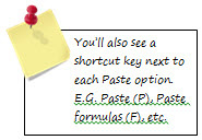
Figure 49  

• • Try it out to see the options you have, as there are several (from right-to-left then down), just enter something in a cell, the copy & paste:

 

• • Paste
• • Paste formulas
• • Paste formulas and number formatting
• • Keep source formatting
• • No borders
• • Keep source column widths
• • Transpose (switch columns to rows and vice versa)
• • Paste values (numbers only, no formulas)
• • Paste values and number formatting
• • Paste values and source formatting
• • Paste formatting only
• • Paste link
• • Paste a Picture
• • Paste a Linked Picture
• • Show Insert Options buttons – This one will appear when you use a Ribbon command to insert rows or columns.

 

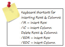
Figure 50  

• • Cut, copy and sort inserted objects with their parent cells – This will make sure that if you resize rows and columns, then any objects (images, controls, etc.) you’ve added will retain their position relative to where you originally placed them. You can also change this for each object in its individual properties.
• • Image Size and Quality
• • Discard editing data – This deletes data Excel saves when you edit images so they can be returned to their original state if you don’t like the changes.
• • Do not compress images in file - Checking this can result in very large image sizes (and therefore large file sizes). By default Excel will compress images so they take up less space.
• • Set default target output to (220, 150 or 96 ppi – pixels per inch)
• • Print
• • High quality mode for graphics
• • Chart
• • Show chart element names on hover (similar to ToolTips)
• • Show data point values on hover (this will show you the value behind a data point on a chart)
• • Display
• • Show this number of Recent Documents (0-50) – This is number of recent file names that will show up in the File, Recent dialog.
• • Ruler Units (Default, Inches, Millimeters, Centimeters) – The default is based on your Windows Regional Settings. In the US it will be Inches.
• • Show all windows in the Taskbar – This will show all of your open workbooks in the Taskbar. If you uncheck this you’ll need to physically move between workbooks to see them. This one is a common question when it’s inadvertently turned off, because all of your workbooks seem to disappear.
• • Show formula bar – This one you might want to turn off if you need to distribute a workbook and don’t want people easily seeing your formulas (more to come when we discuss Worksheet Protection).
• • Show function screen tips
• • Disable hardware graphics acceleration

 

• • For cells with comments, show:
• • No comments or indicators
• • Indicators only, and comments on hover
• • Comments and indicators
• • Default direction – In the US you’ll leave this as Left-to-right.
• • Right-to-left
• • Left-to-right (Default)
• • Display options for this workbook – There is a drop-down on the right of this option that will allow you to choose from any open workbook. The first three options can come in handy when you distribute workbooks and want to minimize what the user sees.
• • Show horizontal scroll bar
• • Show vertical scroll bar
• • Show sheet tabs
• • Group dates I the AutoFilter menus
• • For objects, show:
• • All
• • Nothing (hide objects)
• • Display options for this worksheet – There’s a drop-down on the right of this option that will let you select from any worksheet.
• • Show row and column headers
• • Show formulas in cells instead of their calculated results (you can toggle this in a worksheet with CTRL+`).
• • Show sheet right-to-left – This will reverse the columns in your worksheet and put the last column on your left, column A on the right. Under normal circumstances there’s no reason to do this, but it can be fun to do to unsuspecting co-workers.
• • Show page breaks – Many people find this to be very irritating. If you need to see Page Breaks you’re better off using the Page Break view.
• • Show a zero in cells that have zero values – This is important for worksheets that have formulas that return 0’s. Many times with a lot of information on a sheet you might not want to see a lot of zeros from formulas that haven’t populated yet. This is one option you will probably come to quite a bit.
• • Show outline symbols if an outline is applied – Outlining is a way of compressing information into groups. The outline symbols let you expand or contract those groups, so you wouldn’t want to turn this option off.
• • Show gridlines – Gridlines are the natural dividers between cells and columns. Most times you will apply your own custom gridlines, so while it’s often good to start a worksheet with this option on you may find yourself coming here to turn it off as you get your worksheet completed.
• • Gridline color – You can change the default gridline color if the default gray isn’t spicy enough for you. Note that your choices are limited to the Excel 2003 color palette.
• • Formulas
• • Enable multi-threaded calculation – This takes advantages of multicore processors and lets Excel calculate faster that it could before.
• • Number of calculation threads
• • Use all processes on this computer: (# of processors Windows has identified on your system)
• • Manual (spinner control to change the number)
• • When calculating this workbook - There is a drop-down on the right of this option that will allow you to choose from any open workbook.
• • Update links to other workbooks
• • Set precisions as displayed – This has to do with rounding and how to calculate values as displayed. Unchecking this can cause problems over time as it can affect your data and formula output with regards to multiple value rounding leading to unanticipated results.
• • Use 1904 date system – This is only relevant if you’re using a Macintosh, which uses a different date system. Excel for windows use dates that begin on January 1, 1900. For some odd reason, Mac’s start in 1904.
• • Save external link values – This will save values from formulas that are linked to other workbooks, as well as the formulas. It can come in handy if you send workbooks to other people who might not have the linked workbooks, so when they open your workbook, they’ll see the formula results instead of errors.
• • General
• • Provide feedback with sound – When you do things like insert or delete rows or columns, the action will be accompanied by an alert sound
• • Provide feedback with animation - When you do things like insert or delete rows or columns, you’ll see the action happen. If you turn it off, the action will still take place, it just won’t be as evident until it’s done. It’s generally not an issue unless your graphics card has a hard time keeping up, in which case you might want to turn it off.
• • Ignore other applications that use Dynamic Data Exchange (DDE) – Unless you use multiple monitors this won’t be an issue. If you do though and you want to see Excel on multiple monitors, unchecking this will force each new workbook to open in a new instance of Excel. From there you can drag the separate instances to your different monitors.
• • Ask to update automatic links – When you open a workbook that has links to another you’ll be prompted if you want to update those links. If you do this a lot, this is one of those defaults that you can turn off.
• • Show add-in user interface errors – Unless you deal with a lot of Add-Ins, or at some point you want to create your own, you can leave this alone. By default if there is an error when an add-in tries to load there’s no error message, it just doesn’t load. This will let you know if there are any errors.
• • Scale content for A4 or 8.5 x 11” paper sizes – Excel will automatically try to fit you work to fit in an 8.5 x 11” format, which is the US standard (A4 is European).
• • Show customer submitted Office.com content – This has to do with online content you have posted through OfficeLive. It allows you to open content directly through Excel instead of browsing to a webspace.
• • At start up open all files in – If you have one, or several workbooks you use daily, you can set the path to them here and they will all open each time you open Excel. This isn’t recommended unless you have a workbook that you have opened all day.
• • Web Options – This lets you set some of the options you might want to change if you plan on saving Excel workbooks as web pages, or posting documents to a website.
• • Enable multi-threaded processing – If you have a multi-core processor you’ll probably want to leave this on. If you don’t know what kind of processor you have don’t worry about it.
• • Disable undo for large PivotTable refresh operations to reduce refresh time – Leave this as the default.
• • Disable undo for PivotTables with at least this number of data source rows (in thousands) (spinner control to adjust the default, which is 300) – Leave this as the default. Both of these PivotTable options will improve your performance if you start using them.
• • Create lists for use in Sorts and Fill sequences – This deals with Custom Lists, and of all the General options this is one that you might actually change, especially if you have a business with some fairly repetitive information you need to enter regularly (like department names). You’ll see a command button that allows you to Edit Custom Lists to the right of the option. Clicking it will bring up the following dialog, where you can add your own lists:

 

Figure 51  

• • Custom lists work with the AutoFill handle, which is the little icon at the bottom of an Excel cell when you activate it. If you have a defined list, you only need to enter one of the list values, then grab the fill handle and drag it down or across and Excel will complete the list entries for you for as long as you decide to go (it will repeat the list when it gets to the end of it):

 

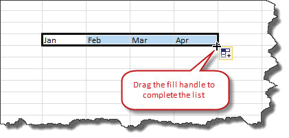
Figure 52  

• • Lotus compatibility
• • Microsoft Excel menu key (set to the Forward Slash - “/” by default, which is the same shortcut launch key that Lotus 1-2-3 uses). The menu key is the same as hitting the Alt key in Excel which will bring up the shortcut keys for each Ribbon Tab and Group.
• • Lotus compatibility Settings – By default, Excel formulas need to be entered with an = sign to start them. These settings allow you to directly enter formulas in Excel without having to preface them with an = sign. It can be handy if you’re inputting a lot of formulas.
• • Customize Ribbon

 

Figure 53  

• • This allows you to add Menu commands to the Ribbon and only display those commands that you want. This feature was not available in Excel 2007, where your only option was to customize the Quick Action Toolbar (QAT). For now the defaults should suffice, but feel free to play around with the options and see what kind of combinations you can come up with to make your experience more enjoyable. As you find yourself getting more comfortable with Excel and its Ribbon commands you may very well find yourself creating your own Ribbon tabs with just the commands you use the most. If you don’t like any changes that you make then just use the Reset button toward the bottom.
• • The first thing to be aware of here is the Choose Commands from option, which allows you to filter the list of available commands. If you don’t see something in the current list of options, you should look here.

 

Figure 54  

• • The second is the Customize the Ribbon option, which will let you choose which Ribbon Tab or Group you want to customize:

 

Figure 55  

• • Quick Access Toolbar
• • As mentioned previously, the Quick Action Toolbar (QAT) is that list of Menu commands that sits above the Ribbon, and it can hold all of your most frequently used commands. If you’re a heavy mouse user then this will probably come in very handy, as it puts everything right up front for you instead of having to go through different Ribbon Tabs/Groups. If you’re a keyboard user, you may never even adjust the default settings. The customize dialog for this is very similar to the Ribbon customization dialog, but it’s a bit simpler. Remember, the default setting is Popular Commands, so if you can’t find something in the list, just change the primary Command selection.

 

Figure 56  

• • Add-Ins
• • As mentioned previously, Add-Ins are additions to what is included natively in Excel. There are Add-Ins that Microsoft creates, and then there are Add-Ins created by third parties. This will show you how to manage Add-Ins if you do find some that are useful for your particular business. This is different than either the Add-Ins Tab on the Ribbon, or the Add-Ins menu on the File Tab, in that this lets you set your Add-In options, where the others expose their functionality.
• • At the top you’ll see a list of active Add-Ins, and below that are inactive Add-Ins. Clicking on any of them will show a description of each one at the bottom of the dialog window.
• • At the bottom there is a drop-down for Manage, which lets you select the type of Add-In you want to work with at the moment:

 

Figure 57  

• • Clicking the Go button will bring up a dialog that shows you the available Add-Ins. You can activate/deactivate them by clicking the check box to the left of the Add-In’s name. If you want to activate an Add-In not in the list, click the browse button and navigate to its location on your computer. Once you do it will appear in the list and you can activate it.
• • Automation is for relatively high-end users and specialized applications. Most users will never use this feature.

 

Figure 58  

• • Trust Center
• • The Trust Center primarily deals with how to tell your computer to respond to workbooks that contain VBA (Visual Basic for Applications) code, be it in the form of code you recorded, wrote, or third party Add-Ins. The links at the top of the dialog will take you to certain Microsoft explanations and offerings. What you’re interested with here is the Trust Center Settings button.

 

 

 

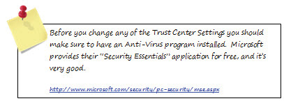
Figure 59  

• • Here you have multiple options:
• • Trusted Publishers – This is only relevant if you have digital certificates issued by a Microsoft third-party certificate issuer. These certificates allow certain documents to bypass security settings as they have been deemed trustworthy. As with Microsoft’s SharePoint application, third-party digital certificates are expensive and usually only used by large corporations. They general don’t play a role in small business applications.
• • Trusted Locations – You’ll want to add certain locations to this list, like your MyDocuments folder, and any other folders you access frequently, otherwise Excel will give you a message that the document didn’t originate from a trusted location and do you want to Enable Content. This will get very old, very fast. You can use the Add New Location button to browse to the folder of your choice.

 

Figure 60  

• • Trusted Documents - When you open a document from an untrusted source, such as one you’ve opened from an untrusted location, Excel will give you the option to permanently trust it.

 

Figure 61  

• • Add-Ins – This Add-Ins area simply gives you the option to require that Add-Ins be signed by a trusted publisher, which requires that they have a Microsoft third-party approved digital signature. If you already know who provided your Add-In and have installed it, it’s unlikely you’ll need to go to this length. It should however, show how serious Microsoft is about protecting you and your information.
• • ActiveX Settings – ActiveX controls are a type of interactive object you can add to your workbooks, like Check Boxes, Radio Buttons, etc. They are all controlled via VBA code, so here’s another instance where Microsoft is trying to protect you from potentially malicious content.

 

Figure 62  

• • Here you have several options:
• • Disable all controls without notification
• • Prompt to enable with restrictions
• • Prompt to enable with minimal restrictions (this option is generally sufficient)
• • Enable all controls without restrictions
• • Macro Settings – These options are designed to give you control over what VBA code can run in Excel (including your own). Generally, if you have an Anti-Virus application installed, you can opt to enable macros, but this is ONLY if you have an Anti-Virus application installed! Otherwise choose the “Disable all macros with notification” option, which will give you the opportunity to allow macros to run or not.

 

Figure 63  

• • There is another setting here called “Developer Macros Settings” with a check box to Trust access to the VBA project object model. If you have any VBA Add-Ins installed you’ll want to make sure that this is checked or your Add-Ins wont’ work.
• • Protected View – Protected view gives you the option of allowing content from workbooks that originate from the Internet or E-Mail attachments. It’s recommended that you leave these options enabled, as you never know what might be in such files. Note that if you have an Anti-Virus application installed it will scan those workbooks first as well.

 

Figure 64  

• • Message Bar – The Message Bar is simply notification that Excel has blocked content. It’s a good idea to leave this option enabled as well.

 

Figure 65  

• • External Content – These are options which you’ll probably have no need to change, as the defaults should be suitable.

 

Figure 66  

• • File Block Settings – This gives you the ability to automatically flag certain workbooks types and open them in protected view. Again, the default settings should suffice, unless you find yourself opening files of a certain type frequently and want to make sure their content is disabled.

 

Figure 67  

• • Privacy Options – These options are largely what you want Excel to check or report back to Microsoft for you. Microsoft collects information from Excel regarding how you use it, crashes, etc., in an effort to improve the application, and they do it for all Office applications. You can opt out of any of it, but you should know that Microsoft doesn’t gather any personal information about you or your data, so it all anonymous.

 

Figure 68  

• • The Document Inspector allows you to inspect a workbook for any personal information prior to distribution and allows you to remove it.
• • The Translation and Research options allow you to set your language preferences for Translation & Research tools when you’re proofing a workbook prior to distribution.

Unit Summary: Basic File Operations & Setting up Excel the way you want it

• • In this lesson you learned about basic file operations, like saving and opening workbooks.
• • You walked through all of Excel’s options for enabling/disabling certain workbook and worksheet features, both features you can use for every instance of Excel and those you can toggle off for specific instances.

Review Questions

1. Name keyboard shortcuts for Opening, Saving/Save As, Closing and creating New workbooks (Extra credit for creating a new template with a shortcut):

a. __________________________________________________

b. __________________________________________________

c. __________________________________________________

d. __________________________________________________

e. __________________________________________________

2. Give examples of valid vs. invalid file names

a. __________________________________________________

b. __________________________________________________

3. How would you create a Read-Only workbook with a Password to open?

a. __________________________________________________

4. What would you do if you didn’t want to display 0 values on a worksheet?

a. __________________________________________________

5. How do you change Excel’s default Font?

a. __________________________________________________

6. What Menu Commands can you add to the Ribbon? What about the Quick Action Toolbar (QAT)?

a. __________________________________________________

b. __________________________________________________

Lesson Assignment – Lesson 2 – Basic File Operations & Setting up Excel the way you want it

Your first assignment is to open a new Excel workbook and start getting familiarized with the default options, including making adjustments to the Ribbon and Quick Action Toolbar (QAT) commands (there is a Notes section below for you to keep track of your observations):