Chapter 8
Introduction to Animation

The best way to learn about animation is to start animating, so you’ll begin this chapter with the classic exercise of bouncing a ball. You’ll then take a closer look at the animation tools the Autodesk® Maya® software provides and how they work for your scene. You’ll do that by throwing an axe. Finally, you’ll tackle animating a more complex system of parts when you bring a locomotive to life.

Learning Outcomes: In this chapter, you will be able to

Set keyframes to establish the movement scheme for an object
Import objects into a scene
Create the feeling of weight and mass for an animated object using scale animation
Read animation curves in the Graph Editor
Differentiate among different animation principles such as squash, stretch, anticipation, and follow-through
Set up a hierarchy for better animation control
Transfer animation between objects
Create text
Create motion trails and animate objects along a path
Set up models for animation
Use selection handles to speed up workflow
Animate objects in time with each other

Keyframe Animation: Bouncing a Ball

No matter where you study animation, you’ll always find the classic animation exercise of creating a bouncing ball. Although it’s a straightforward exercise and you’ve probably seen it a hundred times on the Web and in other books, the bouncing ball is a perfect exercise with which to begin animating. You can imbue the ball with so much character that the possibilities are almost endless, so try to run this exercise as many times as you can handle. You’ll improve with every attempt.

First, you’ll create a rubber ball and create a proper animation hierarchy for it. Then, you’ll add cartoonish movement to accentuate some principles of the animation techniques discussed at the end of the ultra-fabulous Chapter 1, “Introduction to Computer Graphics and 3D.”

Visit the book’s web page for a video tutorial on this ball animation exercise.

Creating a Cartoon Ball

First you need to create the ball, as well as the project for this exercise. Follow these steps:

In a new scene, begin with a poly sphere and then create a poly plane. Scale the plane up to be the ground plane.
Press 5 for Shaded mode.
Move the sphere 1.0 unit up in the Y-axis so that it’s resting on the ground and not halfway through it, as shown in Figure 8-1.

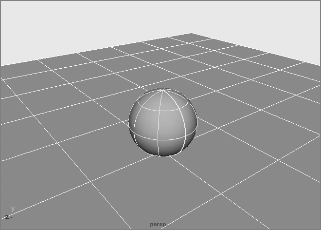
Figure 8-1: Place the ball on the ground.
Choose Modify ⇒ Freeze Transformations to set the ball’s resting height to 0, as opposed to 1. This action sets the ball’s Translate attribute to 0, effectively resetting the object’s values. This is called freezing the transforms. This is useful when you position, scale, and orient an object and need to set its new location, orientation, and size as the beginning state.
Choose File ⇒ Project Window to create a new project. Call the project Bouncing_Ball and place it in the same parent folder as your Solar_System project folder. Choose Edit ⇒ Reset Settings to create the necessary folders in your project and then click Accept. Save the scene file into that project.

Setting Up the Hierarchy

First you’ll set up the ball with three null nodes above it, listed here from the top parent node down: translate, scale, rotate. All the animation will be placed on these three nodes and not the sphere itself. This will allow you to easily animate the ball bouncing, squashing, stretching, and moving forward in space.

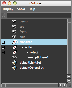
c08f002.tif — **Figure 8-2:** The ball’s hierarchy

Select the sphere and press Ctrl+G to create the first group. In the Outliner, call this new group rotate.
With the rotate node selected, press Ctrl+G to create the scale group, and name it accordingly.
With the scale group selected, press Ctrl+G one last time to create the translate group and name it accordingly. Figure 8-2 shows the hierarchy.

As you animate, you’ll quickly see why you’ve set up a hierarchy for the ball, instead of just putting keys on the sphere.

Animating the Ball

Your next step is to keyframe the positions of the ball using the nodes above the sphere. You’ll start with the gross animation, which is the overall movement scheme, a.k.a. blocking. You’ll move the ball up and down to begin its choreography in these steps:

Press W to open the Translate tool, select the translate node, and move it up to the top of the frame, say about 10 units up in the Y-axis and 8 units back in the X-axis at (–8,10,0). Place the camera so that you’ll have some room to work in the frame.
Instead of selecting the Translate attributes in the Channel Box and RMB+clicking for the Key Selected command, you’ll use hotkeys this time.
Press Shift+W to set keyframes on Translate X, Translate Y, and Translate Z at frame 1 for the top node of the ball (named translate). To make sure your scene is set up properly, set your animation speed to 30fps by choosing Window ⇒ Settings/Preferences ⇒ Preferences to open the Preferences window or by clicking the Animation Preferences button () next to the Auto Keyframe button. In the Settings category of the Preferences window, set Time to NTSC (30fps). A frame range of 1 to 120 is good for now. Figure 8-3 shows the ball’s start position.
Click the Auto Keyframe button () to turn it on; it turns red. Auto Keyframe automatically sets a keyframe at the current time for any attribute that has changed since its last keyframe for the selected object or node.

For the Auto Keyframe feature to work, you first have to set an initial keyframe manually for each of the attributes you want to animate.
Disregarding any specific timing, go to frame 10 and move the ball down in the Y-axis until it’s about one-quarter through the ground plane. Because you’ll be creating squash and stretch for this cartoon ball (see Chapter 1 for a brief explanation), you need to send the ball through the ground a little bit. Then, move the ball about 3 units to the right, to about (–5,–0.4,0). The Auto Keyframe feature sets a keyframe in the X- and Y-axes at frame 10. Remember, this is all on the translate node, not the sphere.
Move to frame 20 and raise the ball back up to about half of its original height and to the right about 2.5 units (–2.5,4,0). Auto Keyframe sets X and Y Translation keyframes at frame 20 and will continue to set keyframes for the ball as you animate.
At frame 30, place the ball back down a little less than one-quarter of the way through the ground and about 2 units to the right, at about (–0.5,–0.3,0).
At frame 40, place the ball back up in the air in the Y-axis at a fraction of its original height and to the right about 1.5 units, at about (1.1,1.85,0).

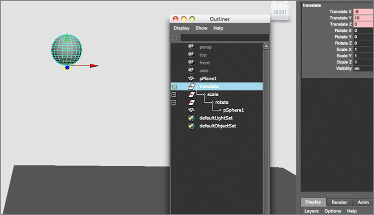
Figure 8-3: Start the ball here and set a keyframe on the translate node.
Repeat this procedure every 10 frames to about frame 110 so that you bounce the ball a few more times up and down and to the right (positive in the X-axis). Make sure you’re decreasing the ball’s height and traveling in X with each successive bounce and decreasing how much the ball passes through the ground with every landing until it rests on top of the ground plane. Open the Graph Editor for a peek into the ball’s animation curves (see Figure 8-4). (Choose Window ⇒ Animation Editors ⇒ Graph Editor.)

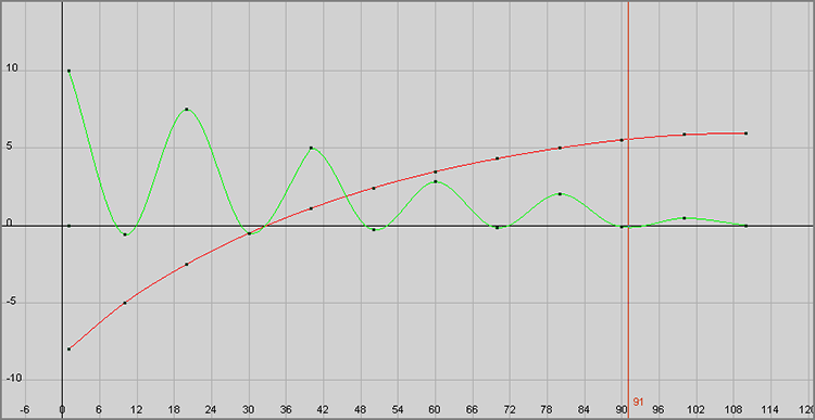
Figure 8-4: The Graph Editor curves for the ball’s translate node

By holding down the Shift key as you pressed W in step 2, you set a keyframe for Translate. Likewise, you can keyframe Rotation and Scale with hotkeys. Here’s a summary of the keystrokes for setting keyframes:

Shift+W Sets a keyframe for the selection’s position in all three axes at the current time
Shift+E Sets a keyframe for the selection’s rotation in all three axes at the current time
Shift+R Sets a keyframe for the selection’s scale in all three axes at the current time

You’ll resume this exercise after a look at the Graph Editor.

The Graph Editor

To use the Maya Graph Editor, select Window ⇒ Animation Editors ⇒ Graph Editor. It’s an unbelievably powerful tool for the animator (see Figure 8-5) to edit keyframes in animation.

Every movement that is set in Maya generates a graph of value versus time, and the Graph Editor gives you direct access to those curves for fine-tuning your animation. The Graph Editor displays animation curves as value versus time, with value running vertically and time horizontally. Keyframes are represented on the curves as points that can be freely moved to adjust timing or value. This window is truly an animator’s best friend. Move a keyframe in time to the right (to be later in the timeline), for example, to slow the action. Move the same keyframe to the left (to be earlier in the timeline) to speed up the action.

The Graph Editor is divided into two sections. The left column, which is much like the Outliner, displays the selected objects and their hierarchy with a listing of their animated channels or attributes. By default, all of an object’s keyframed channels are displayed as colored curves in the display to the right of the list. However, by selecting an object or an object’s channel in the list, you can isolate only those curves that you want to see.

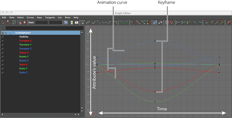
c08f005.tif — **Figure 8-5:** The Graph Editor

Reading the Curves in the Graph Editor

Using the Graph Editor to read animation curves, you can judge an object’s direction, speed, acceleration, and timing. You’ll invariably come across problems and issues with your animation that require a careful review of their curves. Here are a couple of key concepts to keep in mind.

First, the curves in the Graph Editor are like the NURBS curves you’ve modeled with so far. This time, points on an animation curve represent keyframes, and you can control the curvature with their tangency handles. By grabbing one end of a key’s handle and dragging it up or down, you adjust the curvature.

Second, the graph is a representation of an object attribute’s position (vertical) over time (horizontal). So, not only does the placement of the keys on the curve make a big difference, so does the shape of the curve itself. Here is a quick primer on how to read a curve in the Graph Editor and, hence, how to edit it.

In Figure 8-6, the object’s Translate X attribute is being animated. At the beginning, the curve quickly begins to move positively (that is, to the right) in the Z-axis. The object shoots off to the right and comes to an ease-out, where it decelerates to a stop. The stop is signified by the flat part of the curve at the first keyframe at frame 41. The object then quickly accelerates in the negative X direction (left) and maintains a fairly even speed until it hits frame 62, where it suddenly changes direction and goes back right for about 45 frames. It then slowly decelerates to a full stop in an ease-out.

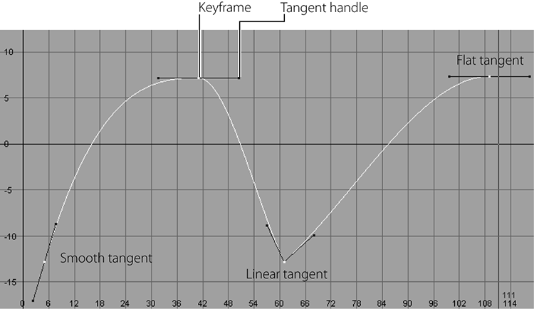
c08f006.eps — **Figure 8-6:** An animation curve

Consider a single object in motion. The shape of the curve in the Graph Editor defines how the object moves. The object shown in Figure 8-7 is moving in a steady manner in one direction.

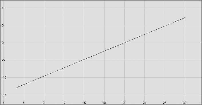
c08f007.tif — **Figure 8-7:** Linear movement

Figure 8-8 shows the object slowly accelerating toward frame 30, where it suddenly comes to a stop. If there is nothing beyond the end of the curve, there is no motion. The one exception deals with the infinity of curves, which is discussed shortly.

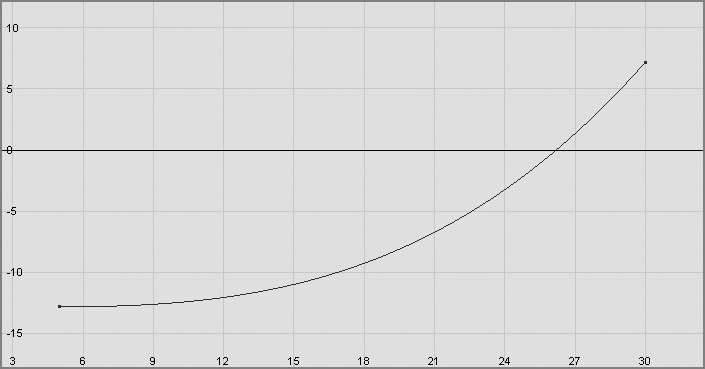
c08f008.tif — **Figure 8-8:** Acceleration (ease-in)

The object in Figure 8-9 begins moving immediately and comes to a slow stop by frame 27, where the curve first becomes flat.

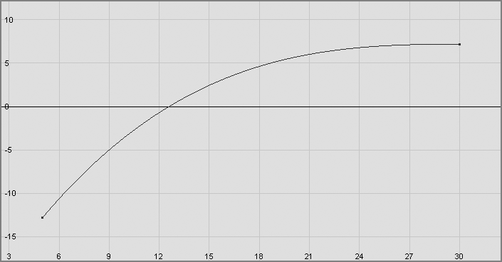
c08f009.tif — **Figure 8-9:** Deceleration (ease-out)

Cartoon Ball

Now, let’s apply what you’ve learned about the Graph Editor to the bouncing ball. Follow these steps:

Open the Graph Editor and look at the ball’s animation curves. They should be similar to the curves shown earlier in Figure 8-4.
Notice how only the X- and Y-axes’ translates have curves, and yet Translate Z has a single keyframe but no curve. It’s from the initial position keyframe you set at frame 1. Because you’ve moved the sphere only in the X- and Y-axes, Auto Keyframe hasn’t set any keys in the Z-axis.
Play back the animation and see how it feels. Be sure to open the Animation Preferences window. Click the Animation Preferences icon () to set the playback speed to Real-Time (30fps). You’ll find this icon in the Playback section in the Time Slider category.
Timing is the main issue now, so you want to focus on how fast the ball bounces and move keyframes to tweak the animation. To move a keyframe, you would select it in the Graph Editor, then press W for the Move tool, and finally MMB+click to move it. But before you move any keys, do the following:
- Watch the motion, and you’ll see that the ball is falling too fast initially, although the second and third bounces should look fine.
- To fix the timing, move the keyframes in the Graph Editor. For the X- and Y-axes, select the keyframes at frame 10 and all the others beyond on both curves. Move them all back two frames. (See Figure 8-10.)
  
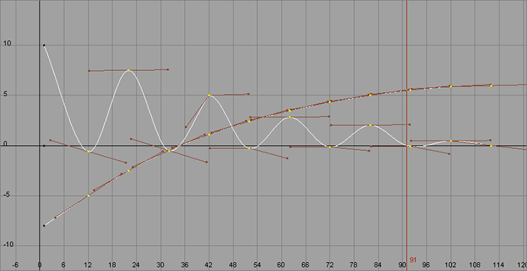
  Figure 8-10: Move all the keyframes for both curves to the right to slow the initial fall by two frames, but leave the timing the same for the rest.

As the ball’s bounce decays over time, it goes up less but still takes the same amount of time (10 frames) to go up the lesser distance. For better timing, adjust the last few bounces to occur faster. Select the keys on the last three bounces and move them, one by one, a frame or two to the left to decrease the time on the last short bounces. (See Figure 8-11.)

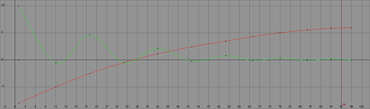
c08f011.tif — **Figure 8-11:** Move the keys to make the final short bounces quicker and the bounce height feel right.

Understanding Timing

In animation, timing is all about getting the keyframes in the proper order. Judging the speed of an object in animation is critical to getting it to look right, and that comes down to timing. Download the file ball_v01.mb from the Bouncing_Ball project on the companion web page, www.sybex.com/go/introducingmaya2015, to get to this point.

When you play back the animation, it seems a bit unrealistic, as if it’s rising and falling on a wave as opposed to really hitting the ground and bouncing back. The problem with the animation is that the ball eases in and out as it rises and falls. By default, setting a key in Maya sets the keyframes to have an ease-in and ease-out in their curves, meaning their curves are smooth like a NURBS curve. For a more natural motion, you need to accelerate the ball as it falls with a sharp valley in the curve, and you need to decelerate it as it rises with smooth peaks. Follow these steps:

In the Graph Editor, select the Translate Y entry in the left panel of the window to isolate your view to just that curve in the editor panel on the right. Select all the landing keyframes (the ones in the valleys of the curve) and change their interpolation from smooth to linear by clicking the Linear Tangents button ().
Likewise, select all the peak keyframes at the ball’s rise and change their tangents to flat by clicking the Flat Tangents icon () to make the animation curve like the one shown in Figure 8-12.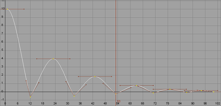

Figure 8-12: The adjusted timing of the bounce
When you play back the animation, the ball seems to be moving more realistically. If you need to, adjust the keys a bit more to get the timing to feel right to you, before you move on to squash and stretch and rotation.

Squash and Stretch

The concept of squash and stretch has been an animation staple for as long as animation has existed. It’s a way to convey the weight of an object by deforming it to react (usually in an exaggerated way) to gravity and motion. You can do this by scaling your object.

Download the file ball_v02.mb from the Bouncing_Ball project on the book’s web page and follow these steps:

Select the scale node (not the sphere!) and select Modify ⇒ Center Pivot. This places the scale pivot point in the middle of the ball.
At frame 9, press Shift+R to set initial scale keyframes on the scale node of the ball, a few frames before the ball impacts the ground.
To initiate squash and stretch, go to frame 12, where the ball hits the floor the first time. With the scale node selected, press R to open the Scale tool; scale the ball down in the Y-axis until it no longer goes through the floor (about 0.6), as shown in the image on the left in Figure 8-13. Set a keyframe for scale by pressing Shift+R.
Move ahead in the animation about three frames to frame 15. Scale the ball up in the Y-axis slightly past normal to stretch it up (about 1.15) immediately after its bounce, as shown in the image on the right in Figure 8-13. Three frames later, at frame 18, set the Y-axis scale back to 1 to return the ball to its regular shape.

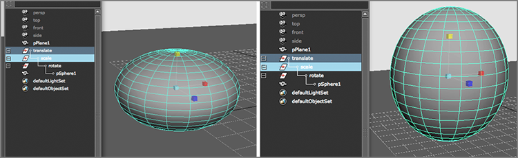
Figure 8-13: Squashing and stretching the ball to react to bouncing on the floor
Scrub your animation, and you should see the ball begin stretching even before it hits the ground. That’s a bit too much exaggeration, so open the Graph Editor and move the Y-axis scale key from 9 to 11. Now, the ball squashes when it hits the floor and stretches as it bounces up.
Repeat this procedure for the remaining bounces, squashing the ball as it hits the floor and stretching it as it bounces up. Remember to decay the scale factor as the ball’s bouncing decays to a stop; the final bounce or two should have very little squash and stretch, if any.

Download the file ball_v03.mb from the Bouncing_Ball project on the book’s web page to get to this point.

Rotation

Let’s add some roll to the ball in these steps:

Select the ball’s rotate node and select Modify ⇒ Center Pivot to set that node’s pivot at the center of the ball.
At frame 1, press Shift+E to set keys for rotation at (0,0,0).
Scrub to the end of your animation (frame 100 in this example) and set a value of –480 for Rotate Z in the Channel Box, as shown in Figure 8-14.

Figure 8-14: Setting a roll for the ball
Open the Graph Editor to see the rotation curve on the ball’s rotate node. It’s a linear (straight) line angled down from 0 to –480. You need the rotation to slow to a stop at the end of the animation, so select the final keyframe and click to make it a flat tangent.

Load the file ball_v04.mb from the Bouncing_Ball project from the companion web page to see an example of the finished bouncing ball. Although the bouncing of this ball looks okay, it could definitely use some finesse, a little timing change, and so on. Open the file, open the Graph Editor, and edit the file to get a feel for animating it in your own style.

Throwing an Axe

This next project will exercise your use of hierarchies and introduce you to creating and refining motion to achieve proper animation for a more complex scene than the bouncing ball. The workflow is simple but standard for properly setting up a scene for animation, also known as rigging. First you’ll model an axe and a target, and then you’ll set up the grouping and pivots for how you want to animate. Then you’ll throw your axe!

Why won’t you throw the NURBS axe you’ve already created and textured? Because later in this chapter, you’ll need it for an exercise on importing and replacing an object in Maya while keeping the animation intact. You’ll see a video tutorial on the book’s website for the axe throwing exercise.

The Preproduction Process

To begin the animation right away, you’ll use a basic axe and bull’s-eye target to focus on animation and technique.

Create a new project: Choose File ⇒ Project Window and click the New button. Place this project in the same folder or drive as your other projects, call it Axe, and click Accept. Click the Animation Preferences button, and set the frames per second to 30fps.

What separates good animation from bad animation is the feeling of weight that the audience infers from the animation. People instinctively understand how nature works in motion. You see an object in motion, how it moves, and how it affects its surroundings. From that, you can feel the essence of its motion, with its weight making a distinct impression on you. As it pertains to animation, that essence is simply called weight. A good feeling of weight in animation depends on timing and follow-through, which require practice.

It’s a good idea first to try an action you want to animate. It may upset the cat if you grab a real axe and start throwing it around your house, but you can take a pen, remove its cap, and lob it across the room. Notice how it arcs through the air, how it spins around its center of balance, and how it hits its mark. Just try not to take out anyone’s eye with the pen. According to some Internet research, the perfect axe throw should contain as few spins as possible.

Animating the Axe: Keyframing Gross Animation

The first step is to keyframe the positions of the axe, starting with its gross animation—that is, the movement from one end of the axe’s trajectory to the other.

Setting Initial Keyframes

Load the scene file axe_v1.mb in the Scenes folder of the Axe project from the companion web page and follow these steps:

Select the axe’s top group node. To make selecting groups such as this easier, display the object’s selection handle. To do so, select the axe’s top node and choose Display ⇒ Transform Display ⇒ Selection Handles. Doing this displays a small cross, called a selection handle (), at the axe’s pivot point. You need only select this selection handle to select the top node of the axe.

You can turn on selection handles for practically any object in Maya—no matter where it is in a group’s hierarchy—whether it’s a child or a parent. Top nodes display as a hollow cross when enabled, and any child nodes appear as a regular cross () when selection handles are turned on.
With the axe selected, go to frame 1 and set a keyframe for the rotation and translation.
Hold down the Shift key, press W for the axe’s translation keyframes, and then press E for the axe’s rotation keyframes for its start position.

Creating Anticipation

Instead of the axe just flying through the air toward the target, you’ll animate the axe moving back first to create anticipation, as if an invisible arm were pulling the axe back before throwing it. Follow these steps:

Go to frame 15.
Move the axe back in the X-axis about 8 units and rotate it counterclockwise about 45 degrees.
The Auto Keyframe feature sets keyframes for the position and new rotation at frame 15.
Because you’ve moved the axe back only in the X-axis and made the rotation only on the Z-axis, Auto Keyframe sets keyframes only for Translate X and Rotate Z. The other position and rotation axes aren’t auto-keyframed because their values didn’t change. Take note of this fact.
Scrub through the animation and notice how the axe moves back in anticipation.

Auto Keyframe inserts a keyframe at the current time for the selected object’s changed attributes only.
Go to frame 40 and move the axe so that its blade cuts into the center of the target.
Notice that you have to move the axe in the X- and Y-axes, whereas before you had to move it back only in the X-axis to create anticipation. This is because the axis of motion for the axe rotates along with the axe. This is an example of the Local axis. The Local axis for any given object shifts according to the object’s orientation. Because you angled the axe back about 45 degrees, its Local axis rotated back the same amount.

The file axe_v2.mb in the Scenes folder of the Axe project from the companion web page will catch you up to this point in the animation.

This last step reveals a problem with the animation. If you scrub your animation now, you’ll notice that the axe’s movement back is different from before, setting a keyframe at frame 40. Why intentionally create a problem like this? Troubleshooting problems in a scene is vital to getting good as a CG animator, so the more you learn how to diagnose problems, the easier production will become.

This is because of the Auto Keyframe feature. At frame 1, you set an initial keyframe for the X-, Y-, and Z-axes of translation and rotation. Then, at frame 15, you moved the axe back in the X-axis only (in addition to rotating it in the Z-axis only).

Auto Keyframe set a keyframe for Translate X at frame 15. At frame 40, you moved the axe in both the X- and Y-axes to strike the target. Auto Keyframe set a keyframe at 40 for Translate X and Translate Y. Because the last keyframe for Translate Y was set at 1 and not at 15 as in the case of Translate X, there is now a bobble in the Y position of the axe between frames 1 and 15.

With the axe selected, open the Graph Editor (choose Window ⇒ Animation Editors ⇒ Graph Editor) to see what’s happening. You should see red, green, and blue line segments running up and down and left and right. You’ll probably have to zoom your view to something more intelligible. By using the Alt key (or the Alt/Option key on a Mac) and mouse-button combinations, you can navigate the Graph Editor much as you can any of the modeling windows.

The hotkeys A and F also work in the Graph Editor. Click anywhere in the Graph Editor window to make sure it’s the active window and press A to zoom all your curves into view. Your window should look something like Figure 8-15.

The curves in the Graph Editor represent the values of the axe’s position and rotation at any given time. The X-, Y-, Z-axes are in their representative red, green, or blue color, and the specific attributes are listed much as they are in the Outliner in the left column. Selecting an object or an attribute on the left displays its curves on the right.

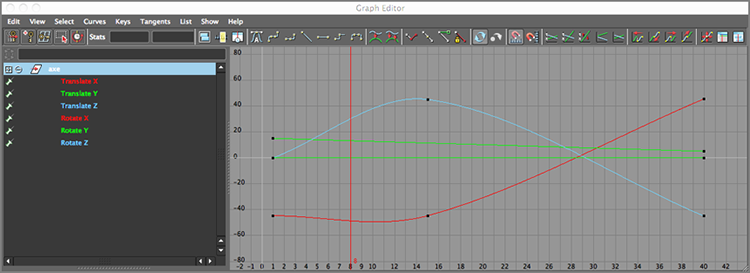
c08f015.tif — **Figure 8-15:** The Graph Editor displays the axe’s animation curves.

You should also notice that the curves are all at different scales. The three rotate curves range in value from about –45 to 45, the Translate Y curve ranges from about 15 to 5, and Translate Z looks flat in the Graph Editor. It’s tough to edit a curve with low values and still be able to see the timings of a larger value curve.

You can select the specific attribute and zoom in on its curve to see it better, or you can normalize the curves so that you can see them all in one view. Click the Enable Normalized Curve Display icon in the top icon bar of the Graph Editor ( c08g007.tif ). The values don’t change, but the curves now display in a better scale in relation to each other so you can see them all together.

Figure 8-16 shows the Graph Editor from Figure 8-15 after the curves have been normalized. Keep in mind that this doesn’t change the animation in the slightest. All it does is allow you to see all the curves and their relative motion. You can denormalize the view by clicking the Disable Normalized Curve Display icon in the Graph Editor ( c08g008.tif ).

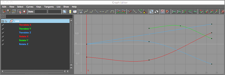
c08f016.tif — **Figure 8-16:** The normalized view in the Graph Editor lets you see all the curves of an animation together in the same scale.

Notice that the curve for Translate Y has keyframes only at frames 1 and 40. The animation dips in the first 15 frames because there is no keyframe at frame 15 like there is for Translate Z. That dip wasn’t there before you set the end keyframe at frame 40.

Continue the exercise by fixing this issue:

Move the first keyframe of Translate Y from frame 1 to frame 15 to fix the dip.
- Press W to activate the Move tool in Maya, or click the Move Nearest Picked Key Tool icon () in the Graph Editor.
- Click the Time Snap On/Off icon () to toggle it on.
- Select the offending Translate Y keyframe at frame 1, and MMB+click and drag it to the right until it’s at frame 15.
Scrub your animation, and the backward movement looks like it did before.

The axe now needs an arc on its way to the target.
Go to the middle of the axe’s flight, frame 27.
Move the axe up in the Y-axis a bit using the green handle of the Tool manipulator.
If the axe is slightly rotated in frame, Auto Keyframe can set a key for both Translate Y and Translate X, although you were perhaps expecting only a key in Translate Y. Because the Move tool is on the axe’s Local axis and because the axe was slightly rotated at frame 27, there is a change in the Y and X positions in the World axis, which is the axis represented in the Graph Editor.
Select the Translate X key at frame 27 in the Graph Editor, if one was created, and press Delete to delete it.
Now you’ll add a full spin to the axe to give the animation more reality and life. You can spin it in one of two ways:
- Go to frame 40, select the axe, and rotate it clockwise a full 360 degrees positive. Auto Keyframe enters a new rotation value at frame 40, overwriting the old value. You should see the Rotate Z curve angle down steeply as soon as you let go of the Rotate manipulator.
- In the Graph Editor, make sure you’re at frame 40, grab the last keyframe on the Rotate Z curve, and MMB+click and drag it down, probably past the lower limit of the window. If you keep the middle mouse button pressed as you move the mouse, the keyframe keeps moving as you move the mouse, even if the keyframe has left the visible bounds of the Graph Editor.
  
  If you hold down Shift as you MMB+click and drag the keyframe to move it in the Graph Editor, the keyframe will move in only one axis (up or down, left or right).
By moving the keyframe down, you change the Rotate Z value to a lower number, which spins the axe clockwise. Before you try that, though, move your Graph Editor window so you can see the axe in the Perspective window. As you move the Rotate Z keyframe down in the Graph Editor, you see the axe rotate interactively. Move the keyframe down until the axe does a full spin.
Play back the animation by clicking the Play button in the playback controls. If your animation looks blazingly fast, open the Animation Preferences window by clicking its icon () and set Playback Speed to Real-Time (30fps).
Now, when you play back the animation, it should look slow. Maya is playing the scene back in real time, but even at 30fps, the scene plays back slowly, and this means that the animation of the axe is too slow.
All you need to do is tinker in the Graph Editor a bit to get the right timing. For a good result in timing, move the first set of keyframes from 15 to 13. Then, grab the Translate Y keyframe at frame 27 and move it to 19. Finally, grab the keyframes at frame 40 and move them all back to frame 25. Play back the scene.

Changing the playback speed of an animation through the Animation Preferences window doesn’t alter the timing of your animation. It only changes the speed at which Maya plays the animation back to you in its windows. To change the playback speed, choose Window ⇒ Setting/Preferences ⇒ Preferences to open the Preferences window, choose Settings ⇒ Working Units, and select the proper setting.

Adding Follow-Through

Load the axe_v3.mb file from the Axe project on the book’s web page or continue with your own file.

The axe is missing weight. You can add some finesse to the scene using follow-through and secondary motion to give more weight to the scene.

In the axe scene, follow-through motion is the axe blade driving farther into the target a little beyond its initial impact. Secondary motion is the recoil in the target as the momentum of the axe transfers into it. As you increase the amount of follow-through and secondary motion, you increase the axe’s implied weight. You must, however, walk a fine line; you don’t want to go too far with follow-through or secondary motion. Follow these steps:

Select the axe in the scene using its selection handle and open the Graph Editor.
Because you’ll add three frames to the end of this animation for follow-through, go to frame 28 (25 is the end of the current animation).
In the Perspective window, rotate the axe another 1.5 degrees in the Z-axis.
Rotating the axe in step 3 moves the axe’s blade down a bit in the Y-axis. To bring the axe back up close to where it was before the extra rotation, move the axe up slightly using the Translate Y manipulator handle. This also digs the axe into the target a little more. You’ll see a keyframe for Translate Y and most probably for Translate X, as well as for Rotate Z.
If you play back the animation, the follow-through doesn’t look good. The axe hits the target and then digs into it as if the action were done in two separate moves by two different animators who never talked to each other. You need to smooth out the transition from the axe strike and its follow-through in the Graph Editor.
Highlight the Rotate Z attribute in the Graph Editor to get rid of the other curves in the window. Figure 8-17 shows the Rotate Z curve of the axe after the follow-through animation is added.

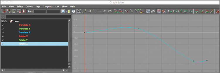
Figure 8-17: The normalized Rotate Z curve of the axe after the follow-through animation
Focus on the last three frames of the curve and zoom into that range only. The curve, as it is now, dips down past where it should and recoils back up a small amount.
When you set keyframes for the axe, you create Bézier splines animation curves in the Graph Editor. These curves stay as smooth as possible from beginning to end. When you set the new keyframe, rotating the axe about 1.5 more degrees for follow-through, the animation curve responds by creating a dip, as shown in Figure 8-17, to keep the whole curve as smooth as possible.

Secondary Motion and Follow-Through

Secondary motion in animation comprises all the little things in a scene that move because something else in the scene is moving. For example, when a superhero jumps from a tall building and his or her cape flutters in the wind, the cape’s undulation is secondary motion.

Follow-through is the action in animation that immediately follows an object’s or a character’s main action. For example, after the superhero lands from their jump, his or her knees buckle a little, and the superhero bends at the waist, reacting to his or her weight as it settles, creating follow-through.

The axe needs to hit the target with force and dig its way in, slowly coming to a stop. You need to adjust the curvature of the keyframes at frame 25 by using the keyframe’s tangents. Tangents are handles that change the amount of curvature influence of a point on a b-spline (Bézier spline). Selecting the keyframe in question reveals its tangents, as shown in Figure 8-18.
Select the Out tangent (handle on the right side of the key) for the Rotate Z attribute’s key at frame 25 and MMB+click and drag it up to get rid of the dip. Notice that the tangency for the In tangent (handle on the left side of the key) also changes.
Press Z to undo your change. You need to break the tangent handles so that one doesn’t disturb the other.
Select the Out handle and click the Break Tangents icon () to break the tangent.
Move the handle up to get rid of the dip so that the curve segment from frame 25 to frame 28 is a straight line, angled down. Figure 8-19 is zoomed into this segment of the curve after it’s been fixed.

Figure 8-18: The tangent handles of a keyframe. The handle to the left of the keyframe is the In tangent, and the handle to the right is its Out tangent.

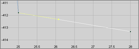
Figure 8-19: Zoomed into the end segment of the Rotate Z animation curve after the dip is fixed

Now, to get the axe to stop slowly as it digs into the target, you need to curve that end segment of the Rotate Z curve to flatten it out.
Grab the last frame to reveal its handles. You can manually move the In handle to make it horizontal, or you can click the Flat Tangents icon () on the left side of the icon bar, under the menus in the Graph Editor.
The curve’s final segment for Rotate Z should now look like Figure 8-20.

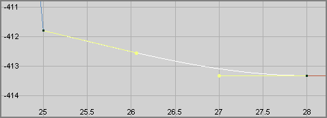
Figure 8-20: Zoomed into the end segment of the Rotate Z animation curve. Notice how the curve now smoothly comes to a stop by flattening out.
Adjust the keyframe tangents similarly for the axe’s Translate Y and Translate X curves, as shown in Figure 8-21.

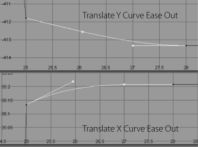
Figure 8-21: Smoothed translate curves to ease out the motion
Play back the animation, and you should see the axe impact the target and sink into it a bit for its follow-through.

Now, you need to polish things up more.

Adding Secondary Motion

Load axe_v4.mb from the Axe project from the book’s web page, or continue with your own scene file. For secondary motion, you’ll move the target in reaction to the impact from the axe’s momentum.

An object in motion has momentum. Momentum is calculated by multiplying the mass of an object by its velocity. So, the heavier and faster an object is, the more momentum it has. When two objects collide, some or all momentum transfers from one object to the other.

In the axe scene’s impact, the axe lodges in the target, and its momentum is almost fully transferred to the target. But because the target is more massive than the axe, the target moves only slightly in reaction. The more you make the target recoil, the heavier the axe will seem.

First, group the axe’s parent node under the target’s parent node by grouping the axe under the target; when you move the target to recoil, it will keep the axe lodged in it. You will use the Hypergraph instead of the Outliner, so let’s take a quick look at its interface first.

The Hypergraph Explained

The Hypergraph: Hierarchy (referred to as just the Hypergraph in this book) displays all the objects in your scene in a graphical layout similar to a flowchart (see Figure 8-22). Select Window ⇒ Hypergraph: Hierarchy to see the relationships between objects in your scene more directly. This window will perhaps be somewhat more difficult for a novice to decipher, but it affords you great control over object interconnectivity, hierarchy, and input and output connections. The Hypergraph: Connections window is technically called the Hypergraph window, but it shows you the interconnections of attributes among nodes as opposed to the node hierarchy in the scene.

Navigating the Hypergraph is the same as navigating any Modeling window, using the familiar Alt key and mouse combinations for tracking and zooming.

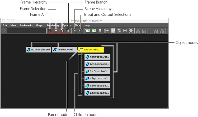
c08f022.eps — **Figure 8-22:** The Hypergraph interface

Continuing the Axe

First you need to reset the target node’s Translate and Rotate attributes to 0 and its Scale attributes to 1.

To freeze the transforms, select the parent target node and then choose Modify ⇒ Freeze Transformations.
Select Window ⇒ Hypergraph: Hierarchy. MMB+click and drag the axe node to the target node in the Hypergraph to group the axe node under the target node. This can also be done in the Outliner.
Go to frame 25, the moment of impact, and set the position and rotation keyframes on Target.
Go to frame 28, rotate the target node in the Z-axis about 2.5 degrees, and move it up and back slightly in the Y- and X-axes, as shown in Figure 8-23.

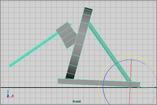
Figure 8-23: The front-panel display of the target reacting to the impact of the axe
Go to frame 31. Rotate the target node back to 0 in the Z-axis, move it down to 0 in the Y-axis, and move it back a bit more in the X-axis.
Go to frame 35 and repeat step 4, but move it only half as much in Rotate Z, Translate X, and Translate Y.
Go to frame 40 and repeat step 5, but move Target back only slightly in the X-axis.

If you don’t freeze the transforms on the target’s parent node before grouping the axe under it, the axe’s animation will change and yield undesirable results.

The preceding steps should give you an animation similar to axe_v5.mb in the Axe project from the companion web page.

Path Animation

As an alternative to keyframing the position of the axe, you can animate it on a path. Path animation allows you to assign an object to move along the course of a curve, called a path.

Load axe_v6.mb from the Axe project from the companion web page. This is the finished axe animation, but the translation keys have been deleted, though the rotation keys and everything else are intact. You’ll replace the translation keyframes with a motion path instead. There is an arched curve in this scene called pathCurve that was already created for you using the CV curve tool. Look how nice I am to you!

Once you open the scene (axe_v06.mb), scrub the animation and you’ll see that the axe spins around; it and the target recoil at the moment of impact, but the axe doesn’t actually move. There is also a curve in the scene that represents the eventual motion of the axe.
Select the axe node in the Outliner (Figure 8-24) and then Shift+select the path curve. In the Animation menu set, choose Animate ⇒ Motion Paths ⇒ Attach To Motion Path .

Figure 8-24: Select the Axe project’s group node.
In the option box, turn off the Follow check box.
The Follow feature orients the object on the path so that its front always points in the direction of travel. This will interfere with the axe’s motion, so you’ll leave it off. Click Apply, and now the axe will follow the line from end to end between frame 1 and frame 60. Of course, you have to adjust the timing to fit better, as with the original axe animation.

The file axe_path_v1.mb in the Axe project will bring you up to this point.
Select the axe node and open the Graph Editor to see the axe’s curves. There is a purple curve called motionPath1.U Value curve that replaces the translation curves. On the left side of the Graph Editor, select the motionPath1.U Value curve to display only that. Zoom into it. (Press A to view all.)
The curve is an ease-in and ease-out curve from 1 to 60. You need the axe to hit at frame 25, so move the end of that curve to frame 25 from frame 60. Then use the tangent handle to shape the end of the curve to be more like Figure 8-25. This will add acceleration to the end of the curve for more of a punch on the hit.

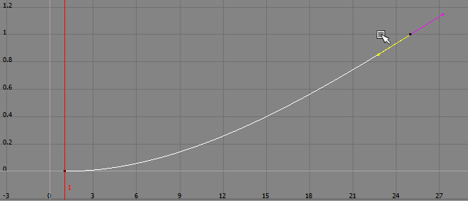
Figure 8-25: Set the last key to frame 25 and reshape the curve at the end.
Scrub the animation until the axe moves all the way back (frame 4). You’ll add a keyframe here to help retime the backward movement. Select the purple U Value animation curve and then select the Insert Keys tool () in the top-left corner of the Graph Editor. MMB+click the curve to create a key at frame 4. (You can MMB+click and then drag the cursor to place the key precisely at frame 4 before releasing the mouse button.)
Move this new keyframe to frame 7. Scrub the animation, and the timing is just about right. You’ll have to adjust the tangents a bit to make the axe move more like before, but the movement is essentially there with path animation.

The file axe_path_v2.mb in the Axe project will bring you up to this point.

Path animation is extremely useful, especially for animating an object along a particular course. By adjusting the resulting animation curve in the Graph Editor, you can easily readjust the timing of the path animation, and you can always adjust the shape of the path curve itself to change the motion of the object. A good path animation exercise is to reanimate the Solar_System exercise with paths instead of the keyframes you set on the rotations.

Replacing an Object

It’s common practice to animate a proxy object—a simple stand-in model that you later replace. The next exercise will show you how to replace the axe you already animated with a fancier NURBS model and how to copy an animation from one object to another.

Replacing the Axe

Load the scene file axe_v5.mb from the book’s web page. Now, follow these steps:

Choose File ⇒ Import.
Locate and import the Axe_Replace.ma scene file from the Scenes folder of the Axe project from the companion web page. The new axe appears at the origin in your scene.

Transferring Animation

Transferring all the properties and actions of the original axe to a new axe requires some setup. Follow these steps:

Move the pivot on the new axe to the same relative position as the pivot on the original animated axe (up toward the top and a little out front of the handle, just under the blade). This ensures that the new axe has the same spin as the old axe. Otherwise, the animation won’t look right when transferred to the new axe. Figure 8-26 shows the pivot’s location.

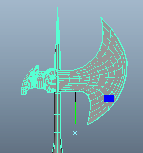
Figure 8-26: Place the pivot point on the new axe here.
Use grid snap to place the top node of the new axe at the origin.
Choose Display ⇒ Transform Display ⇒ Selection Handles to turn on the selection handle of the new axe.
Go to frame 1. Select the original axe’s axe node, open the Graph Editor, and choose Edit ⇒ Copy.
Select the new axe to display its curves in the Graph Editor. It has no curves to display yet. With the new_Axe node selected in the Graph Editor, choose Edit ⇒ Paste. As shown in Figure 8-27, the new axe is slightly offset from the original axe.

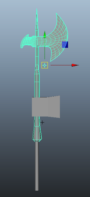
Figure 8-27: The new axe placed next to the original

When you copy and paste curves in the Graph Editor, make sure you’re on the first frame of the animation. Pasting curves places them at the current frame. Because the animation of the original axe started at frame 1, make sure you’re at frame 1 when you paste the curves to the new axe.
You have to move the new axe to match the original, but because it’s already animated, you’ll move it using the curves in the Graph Editor. With the new axe selected, in the Graph Editor select the Translate Y curve; move it down to match the height of the original axe.
Scrub the animation to see that the new axe has the same animation except at the end when it hits the target. Remember that you grouped the original axe under the target node for follow-through animation. Place the new axe under this node as well.
The file axe_v7.mb in the Axe project from the book’s web page has the new axe imported and all the animation copied to get you caught up to this point.
After you scrub the animation and make sure the new axe animates properly, select the original axe’s node and delete it.

Animating Flying Text

It’s inevitable. Sooner or later, you will need to animate a flying logo or flying text. Animating flying text—at least, the way you’ll do it here—can show you how to animate pretty much anything that has to twist, wind, and bend along a path; this technique isn’t just for text.

You’ll need to create the text, so follow these steps:

In a new scene, select Create ⇒ Text . In the option box, enter your text and select a font to use (see Figure 8-28). In this case, stick with Times New Roman. Set Type to Bevel.

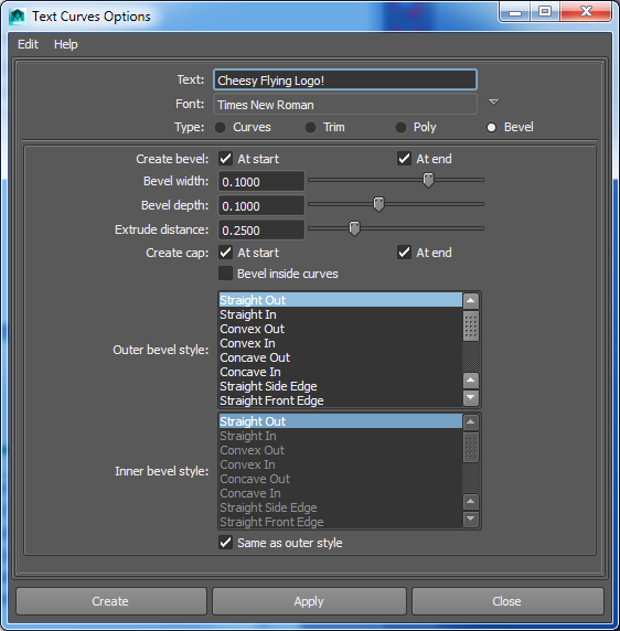
Figure 8-28: The Text Curves Options box

Setting the Type attribute to Poly for your text creates curve outlines for the text and planar faces for the letters, for a flat-text effect. Setting the Type Creation option to Curves gives you just the curve outlines. Finally, using Trim to create your text makes the letters out of flat planar NURBS surfaces. However, no typographical surface history is created with text. To allow you to edit the text, you must re-create the text and/or font as needed.
Leave the rest of the creation methods at their defaults. Doing so creates the text as beveled faces to make solid text with thickness.
When you have the text, you need to create a curve for it to animate along. Using either the CV or EP Curve tool, create a winding curve like a rollercoaster for the logo, shown with the text in Figure 8-29.

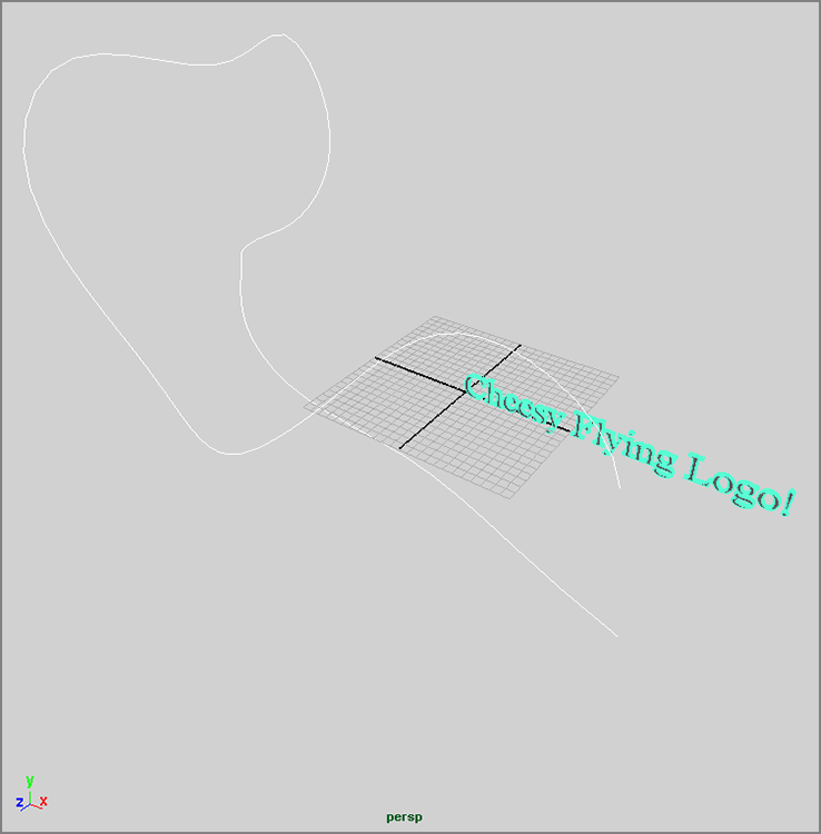
Figure 8-29: Create a curve path for the text to follow.
Just as you did with the axe exercise, you’ll assign the text object to this curve. Set your frame range to 1–100. Select the text, Shift+select the curve, and, in the Animation menu set, choose Animate ⇒ Motion Paths ⇒ Attach To Motion Path . Set Front Axis to X and Up Axis to Y, and select the Bank check box, as shown in Figure 8-30.

Figure 8-30: The Attach To Motion Path Options box

Depending on how you create your curve and text, you may need to experiment with the Front Axis and Up Axis attributes to get the text to fly the way you want.
Orbit the camera around to the other side, and you can see the text on the path, as shown in Figure 8-31. In the Attribute Editor for the motion path, notice the U Value attribute: This is the position of the text along the curve from 0 to 1. Scrub the animation, and the text should glide along the curve.
The text isn’t bending along with the curve at all yet. To accomplish this, you need to add a lattice that bends the text to the curvature of the path. Select the text object, and choose Animate ⇒ Motion Paths ⇒ Flow Path Object .
In the option box for the Flow Path Object, set Divisions: Front to 120, Up to 2, and Side to 2, and select Curve for Lattice Around. Make sure the Local Effect box is unchecked. Doing so creates a lattice that follows the curve, giving it 120 segments along the path. This lattice deforms the text as it travels along the path to the curvature of the path.
Scrub your animation, and you see a fairly strange result: Parts of the text explode out from the lattice, as shown in Figure 8-32.
The geometry is going outside the influence of the lattice. To fix the situation, select the lattice and base node; then scale up the lattice and its base node together to create a larger size of influence around the path (see Figure 8-33).

Scrub your animation to check the frame range and how well the text flies through the lattice. When the lattice and its base are large enough to handle the text along all of the path’s corners and turns, voilà—Cheesy Flying Logo! (See Figure 8-34.)

c08f031.tif — **Figure 8-31:** The text is on the path.

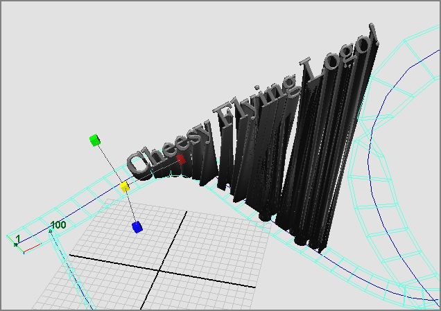
c08f032.tif — **Figure 8-32:** The geometry doesn’t fit the lattice well. Ouch!

c08f033.tif — **Figure 8-33:** Scale the lattice and its base node to accommodate the flying text.

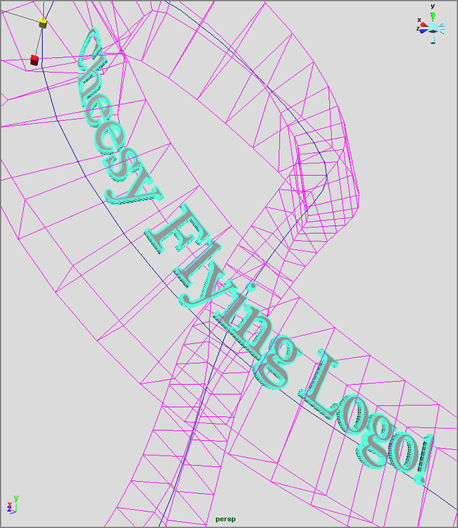
c08f034.tif — **Figure 8-34:** Cheesy Flying Logo! makes a nice turn.

Animating the Catapult

As an exercise in animating a system of parts of a model, you’ll now animate the catapult from Chapter 4, “Beginning Polygonal Modeling.” You’ll turn its winch to bend back the catapult arm, which shoots the projectiles, and then you’ll fire and watch the arm fly up.

Let’s get acquainted with the scene file and make sure its pivots and hierarchies are set up properly. The scene file catapult_anim_v1.mb in the Catapult_Anim project from the companion web page has everything in order, although it’s always good to make sure. Figure 8-35 shows the catapult with its winch selected and ready to animate.

Get a sense of timing put down for the winch first and use that to pull back the arm to fire. Follow these steps:

Select the Winch group with its selection handle. At frame 1, set a keyframe for rotation. If the selection handle isn’t turned on, select Winch from the Outliner and turn on the selection handle by choosing Display ⇒ Transform Display ⇒ Selection Handles. To keep it clean as you go along, instead of pressing Shift+E to set a key for all three axes of rotation, select only the Rotate X attribute in the Channel Box, right-click to open the context menu, and choose Key Selected. There only needs to be rotation in X for the winch.
Jump to frame 60. Rotate the winch backward a few times or enter –400 or so for the Rotate X attribute.
Open the Graph Editor, ease in the curve a bit, and ease out the curve a lot so that the rotation starts casually but grinds to a stop as the arm becomes more difficult to pull back.

Figure 8-35: The catapult’s winch is ready to animate.

Because animating a rope is a fairly advanced task, the catapult is animated without its rope; however, the principle of an imaginary rope pulling the arm down to create tension in the arm drives the animation.
To accentuate the more difficult winding at the end, add a key to the X-axis rotation through the Graph Editor. To do so, select the curve and click the Insert Keys Tool icon () in the upper-left corner of the Graph Editor.
MMB+click and drag to place a new keyframe positioned at frame 42. You can always drag the key back and forth on the curve to place it directly at frame 42. It may help to turn on key snapping first. (See Figure 8-36.)

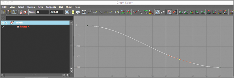
Figure 8-36: Insert a keyframe at frame 42.
Move that keyframe down to create a stronger ease-out for the winch. Be careful not to let the curve dip down so that the winch switches directions. Adjust the handles to smooth the curve. You can also add a little recoil to the winch by inserting a new keyframe through the Graph Editor at frame 70. (See Figure 8-37.)

Figure 8-37: Creating a greater ease-out and adding a little recoil at the end

Animating with Deformers

It’s time to animate the arm coiling back, using the winch’s timing as it’s driving the arm. Because the catapult’s arm is supported by a brace and the whole idea of a catapult is based on tension, you have to bend the arm back as the winch pulls it.

You’ll use a nonlinear deformer, just as you did in the axe head exercise in Chapter 5, but this time, you’ll animate the deformer to create the bending of the catapult arm. Follow these steps:

Switch to the Animation menu set. Select the Arm1 group, and choose Create Deformers ⇒ Nonlinear ⇒ Bend to create a Bend deformer perpendicular to the arm. Select the deformer and rotate it to line it up with the arm, as shown in Figure 8-38.

Figure 8-38: Align the Bend deformer with the catapult arm.
With the Bend deformer selected, look in the Channel Box for bend1 under the Inputs section, and click it to expand its attributes. Try entering 0.5 for Curvature. More than likely, the catapult arm will bend sideways. Rotate the deformer so that the arm is bending back and down instead, as shown in Figure 8-39.

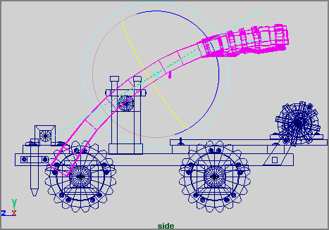
Figure 8-39: Orient the Bend deformer to bend the arm back and down.
You don’t want the arm’s base to bend back, just the basket side. You want it to bend at the brace point, not in the middle where it is now. Move the deformer down the length of the arm until the middle lines up with the arm’s support brace.
To prevent the bottom of the arm from bending, change the Low Bound attribute to 0. To keep the basket from bending, set the High Bound attribute to 0.9.
Instead of trying to match the speed, ease-in, and ease-out of the winch, set the gross keyframes for the arm pulling back first. Reset Curvature to 0, and set a key for Curvature at frame 1. (Select bend1’s Curvature in the Channel Box, right-click, and choose Key Selected from the context menu.)

The Low Bound and High Bound attributes control how far up and down the deformer the object is affected. The Envelope attribute for a deformer governs how much the object is affected overall, with 0 not affecting the geometry at all.
Go to frame 60 and set Curvature to 0.8. If Auto Keyframe is turned on, this sets a keyframe; otherwise, set a key manually. (See Figure 8-40.)

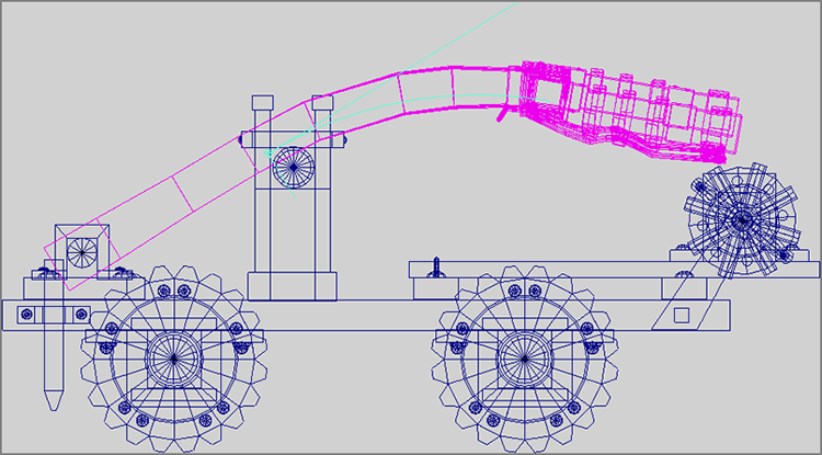
Figure 8-40: Bend the arm back at frame 60 and set a keyframe.
If you play back the animation, notice that the way the winch winds back and the way the arm bends don’t match. In the Graph Editor, you can adjust the animation curve on the Bend deformer to match the winch’s curve.
Insert a key on the Curvature curve at frame 42 and move it up to match the curvature you created for the winch.
Insert a new key at frame 70 and make the arm bend back up slightly as the winch recoils. Set Curvature to about 0.79 from 0.8. (See Figure 8-41.)

Figure 8-41: Try to match the relative curvature of the winch’s animation curve with the Bend deformer’s animation curve.
Go to frame 90 and set a key again for Curvature at 0. Set a key at 0.82 for frame 97 to create anticipation and then keyframe at frame 103 to release the arm and fire the imaginary payload with a Curvature of –0.8.
Add some rotation to the arm for dramatic effect. At about frame 100, during the release, the arm is almost straight. Select the Arm1 group and set a rotation key on the X-axis. Go to frame 105 and rotate the arm 45 degrees to the left in the X-axis. If the starting rotation of the arm is at 30 (as it is in the sample file), set an X-axis rotation key of 75 at frame 105.
Notice that the arm is bending strangely now that it’s being rotated. It’s moving off the deformer, so its influence is changing for the worse. To fix this, go back to frame 100 and group the deformer node (called bend1Handle) under the Arm1 group, as shown in Figure 8-42. Now it rotates along with the arm, adding its own bending influence.

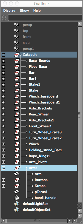
Figure 8-42: Group the deformer node under the Arm1 group node.
Work on setting keyframes on the deformer and the arm’s rotation so that the arm falls back down onto the support brace and quivers until it becomes straight again. The animation curve for the Bend deformer should look like Figure 8-43. The rotation of the arm should look like Figure 8-44. Remember to make the tangents flat on the keys where the arm bounces off the brace and at the peaks, like the ball’s bounce from earlier in the chapter.

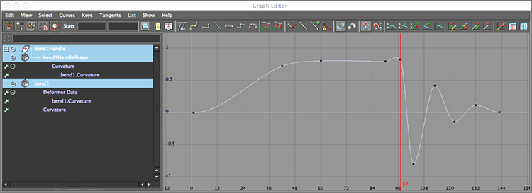
Figure 8-43: The animation curve for the arm’s vibration back and forth as it comes to a rest

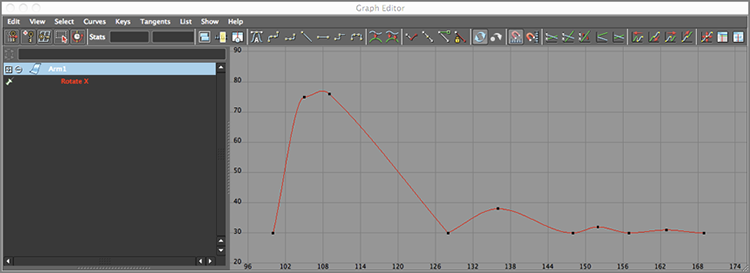
Figure 8-44: The animation curve for the arm’s rotation as it heaves up and falls back down, coming to an easy rest on the brace

The file catapult_anim_v2.mb will give you a good reference to check out the timing of the arm bend and rotation. Here are some items you can animate to make this a complete animation:

Spin the winch around as the arm releases, as if its rope is being yanked away from it.
Animate the entire catapult rocking forward and backward as the arm releases, similar to the way a car rocks when you jump onto the hood.
Move the catapult forward on a road, spinning its wheels as best you can to match the distance it travels.
Design and build your own catapult and animate it along the same lines.

Summary

In this chapter, you began to learn the fundamentals of animating a scene. Starting with a bouncing ball, you learned how to work in the Graph Editor to set up and adjust timing as well as how to add squash and stretch to the animation. The next exercise, throwing an axe, expanded on your experience of creating timing in the Graph Editor and showed you how to add anticipation, follow-through, and secondary motion to your scene. You then learned how to animate the axe throw using path animation. You went on to learn how to replace a proxy object that is already animated with a different finished model and how to transfer the animation. Finally, you used the catapult to animate with deformers and further your experience in the Graph Editor.

Animating a “complex” system, such as a catapult, involves creating layers of animation based on facets of the mechanics of the system’s movement. With the catapult, you tackled the individual parts separately and then worked to unify the animations. You’ll use rigging concepts in the next chapter to automate some of that process for a locomotive. The same is true of the Bouncing_Ball and Axe_Throwing exercises. The different needs of the animation were addressed one by one, starting with the gross animation and ending with finishing touches to add weight.

Animation is the art of observation, interpretation, and implementation. Learning to see how things move, deciphering why they move as they do, and then applying all that to your Maya scene is what animation is all about.