1 Introduction
GDP as a comprehensive scorecard of a country’s economic health is one of the most important and widely researched economic indicator. It represents the market value of all goods and services produced by an economy during a given period [14]. Economists are interested in measuring the overall amount of goods and services produced in a country over a given period, which is not affected by the changes in prices. Real GDP considers the impact of inflation, allowing to compare the economic output of two countries or two different periods and to evaluate, whether a certain economy is expanding or contracting [15].
In literature, many authors are interested in exploring or forecasting GDP growth. For example [19] used panel data approach to explain the real GDP using the correlation with employment. Sorić [21] has discovered the time-varying impact of consumer confidence on GDP growth. His empirical analysis was based on a dataset of 11 new EU Member States. Taş et al. [24] analyzed the relationship between economic growth and macroeconomic indicators of the EU countries using panel data approach. They used 10 years data and they examined the effects of eleven macroeconomic indicators on GDP. The forecast of the German GDP is reported in [17, 18]. These authors propose alternative methods for forecasting quarterly GDP with monthly factors. Another approach to predict French GDP used Bec and Mogliani in their paper [1]. These authors investigate forecast combination and information pooling, in the context of France’s GDP prediction in real time with monthly survey opinions. Rusnák [16] describes a Dynamic Factor Model to predict Czech GDP using multiple historical data over the period from 2005 to 2012. Bjørnland et al. [2] examined the existence of a systematic influence in the co-movement across countries to improve the forecast accuracy at the national level. They used dynamic factor model and their results show that exploiting the informational content in a common global business cycle factor improves the forecast accuracy across a large panel of countries. Soares et al. [20] used wavelet analysis to analyze inflation dynamics convergence in the Euro area. They discover that before Euro adoption the synchronization pattern was stronger in the 11 countries that first adopted the Euro as after Euro adoption. Development of GDP and inflation is also necessary for service-oriented enterprises as was described in [7, 9, 12, 13, 22, 23].
The main purpose of this chapter is to analyze the nominal GDP and inflation to point out the co-movements and the heterogeneity in its values. We researched the first member states as well as all the countries of the EU together by employing statistical methods. The paper contains descriptive statistics and principal component analyses for both the longer and shorter period. The results indicate how many principal components are needed to keep the original variability of the data. They also reveal the problematic countries and years. Additionally, in the longer period (1967–2015) we employed linear regressions. The established regression models for France and Luxembourg enable to explain the relationship between these countries nominal GDP and the principal components.
Describe the developments of inflation and GDP in the examined periods by descriptive statistics.
Identify the main factors using the PCA analysis, which express the inflation and GDP in the analyzed EU countries.
Compare the interdependence of the EU countries that were not affected by changes in their political system as well as the interdependence of the countries in Central and Eastern Europe, who became independent states after the end of the socialist regime.
Identify problematic countries, based on the results from the PCA analysis.
Reveal the problematic years based on the results from PCA analysis.
Determine the linear regression models for France and Luxembourg to be able to assess the relationship between their inflation/GDP and the principal components in the period between 1967 and 2015.
2 Inflation
The growth of the price level has been one of the main subjects of economic researches during the development of the economic thinking. In the period of mercantilism, economists J. Locke and T. Mun found a positive correlation between the amount of money in the economy and the price level. The views of economists are broadly consistent with the fact that the rate of inflation in the long run depends on the growth of money supply, but we also should consider the growth rate of real output. The most frequent topics in the field of inflation are its causes, the impact on individual subjects and the ways to remove the negative trends and the associated costs.
During inflation the value of money declines and for the same amount of money it is possible to buy fewer goods and services. Increases in the price level also causes increased incomes. However, real income will not be affected by the changes in the price level in case that it changes proportionally in the same way with the prices.
Inflation represents an increase in the economy’s overall price level, leading to a decline in the purchasing power of money. There are various reasons why faster growth of aggregate demand compared to the growth of aggregate supply causes inflation. The imbalance of the aggregate demand and supply can be linked to the state’s budget deficit, the increase of the interest rates and the foreign demand.
Inflation can be associated with deflation, which is a continuous decline in the price level of goods and services. It is important to distinguish it from the phenomenon of falling prices in one economic sector, which is called disinflation. In addition, deflation can also have a positive impact on the economy, when lower prices increase the real income.
There are two reasons why a high level of inflation is not perceived as a desirable target for central banks. The first is that it is obviously difficult to reduce nominal wages. Deflation trap occurs when low levels of aggregate demand causes the price levels to fall, leading to a negative inflation. In this situation, the central bank’s aim is to stimulate the economy by decreasing the nominal interest rates. The combination of low interest rates with a deflation results positive real interest rates, which is not the best solution to stimulate the demand in the private sector. The demand will continue to decline, so deflation does not require the central bank’s active co-operation.
2.1 Measuring the Inflation
Inflation is an increase in the overall price level. It causes a decline in the real value and the purchasing power of money. Inflation is measured by the rate of inflation which is expressed as a percentage change in the price level. We distinguish various price indices that are used to monitor the price level in the economy according to Čaplánová and Martincová [5] as Consumer Price Index (CPI), GDP deflator, Producer Price Index (PPI) and Harmonized Index of Consumer Prices (HICP). Each of them reports the price level from a different perspective.

As wrote Gerdesmeier in [6], inflation expressed by a certain price index is only an approximate measure of the economic situation. Over the time, consumers try to replace more expensive products with cheaper ones and the consumer basket becomes no longer representative. Another challenge is how to include the product quality developments in the price index. An increase in the price of a product due to an improvement in its quality is not considered to be the cause of inflation because it does not reduce the purchasing power of the money.
The CPI index is used to monitor the price changes in the short term. Any increase in the consumer prices is interpreted as an increase in inflation. This price index does not take into account the price increases due to improvements in the quality of the products. This means that the estimated rate of inflation can be higher than its actual value. It is important to mention that an increase in the nominal prices is similarly followed by an increase in the nominal wages. At the end, the real price of the products remains unchanged. The methodology of putting together and the constant updates of the consumer basket play an important role in revealing the inaccuracies.
The Harmonized Index of Consumer Prices, initiated by EUROSTAT, serves to point out the differences in national consumer habits. HICP is calculated differently from the other price indices. First, it is calculated from a smaller consumer basket. It considers only the current consumption expenses. For example, it excludes the expenses related to the cost of living in family houses. The main difference between the HICP and CPI is the calculation of weights. Additionally, the HICP includes the expenditures of the countries households. Expenditures of expats living in the country whose HICP is measured are also included in [11]. This index does not involve the spending of the households based outside their home country. In contrary the CPI considers only the expenditures of the national households excluding expat households.
3 GDP
In the past, to measure the overall economic activity economists needed to combine a wide range of information, for example data about iron shipments or sales in the department stores. As Blanchard and Johnson wrote in [3], the national income accounts were not reported before the Second World War. Similarly, the first release of the aggregate output data was in 1947 in the US. Of course, we can find earlier data but these had been compiled retrospectively.
GDP is the value of all final goods and services produced in a country over a given period.
GDP is the value added in the economy.
GDP is the sum of each subject’s income in the economy over a given reference period.


If the disposable income increases, then a household will own more money that they can invest, resulting their consumption to increase. This and similar equations economists consider as a behavioral because it explains the consumers demeanor.
The private domestic investments also form a large proportion of the GDP, including asset purchases. As an example, they occur when firms expand their capacity by buying plant, property and equipment. These investments do not include purchases of different shares on the secondary market, since they are not considered as an investment [4].
Government spending consist of expenditures for numerous purposes, for example wages for employees in the public sector, investments in the infrastructure expected to generate benefits in the future. Transfer payments e.g. unemployment or child benefits are spending that are not intended to conduct transactions of goods and services, but instead they serve as a transfer of money. In a macroeconomic context they can be explained as negative taxes [14].
Export represents the purchase of goods and services produced in the home country by foreign subjects. Conversely, import is a purchase of goods and services originating from another country by domestic subjects. The difference between export and import is called net export or trade balance. There can occur two situations based on the trade balance. If export exceeds the country’s import, it results a trade surplus. Otherwise, higher import than export is followed by a trade deficit as is wrote in [3].
Another term which we introduce is the GDP deflator, used to monitor the prices changes in the long term. The data are reported on a year-on-year basis. It is an aggregate price index, including all the goods and services produced in the economy during a given year. GDP deflator is appropriate when compiling time series from the price changes as well as comparing countries over a long period [5].

In the basis year the value of the GDP deflator is equal to 100 as the values of the nominal and real GDP in that year are identical (see [4]).
4 Data and Results
We analyzed the annual CPI index and the nominal GDP denominated in USD. The data were obtained from the World Bank’s (2016) [25], publicly available database. For the data analysis we employed the statistical software SAS Enterprise Guide.
The EU countries were divided based on the changes that took place in their political system. The developments of these macroeconomics indicators were examined during two periods. In the case of GDP, the first analyzed period was from 1967 to 2015. During this period, we analyzed the first member countries (except Germany), i.e. countries, that were not affected by socialism and the countries that joined the EU before 1995 inclusive. This analysis included the following 14 countries of the EU: Austria, Belgium, Denmark, Finland, France, Greece, Ireland, Italy, Luxembourg, the Netherlands, Portugal, Spain, Sweden and the United Kingdom. The second period spans from 1995 to 2015, where we analyzed the development of the nominal GDP in each country of the EU. Concerning the inflation, the analyzed period from 1967 to 2015 includes the original member states and the countries, which joined the EU before 1995 excluding Germany, the United Kingdom and the countries which were one of the succession states of the socialist regime. Additionally, this analysis contains Malta and Cypress. The period between 1994 and 2015 includes all the countries of the EU.
Principal Component Analysis (PCA) [8, 10] was used to find main driver in GDP and CPI of the EU members states in this chapter. We discover some principal components (PCs) for each sample data. Linear regression models are given for selected countries to predict their GDP and inflation based on PCA results.
4.1 Nominal GDP During the Period from 1967 to 2015
Descriptive Statistics of Nominal GDP for the First EU Member Countries (except Germany). Data period from 1967 to 2015
Country | Mean | Standard deviation |
|---|---|---|
AUT | 1.82E+11 | 1.39E+11 |
BEL | 2.26E+11 | 1.65E+11 |
DNK | 1.50E+11 | 1.10E+11 |
FIN | 1.18E+11 | 8.70E+10 |
FRA | 1.28E+12 | 9.00E+11 |
GRC | 1.24E+11 | 9.93E+10 |
IRL | 9.06E+10 | 9.39E+10 |
ITA | 1.03E+12 | 7.36E+11 |
LUX | 2.04E+10 | 1.99E+10 |
NLD | 3.77E+11 | 2.88E+11 |
PRT | 9.97E+10 | 8.37E+10 |
ESP | 5.86E+11 | 5.01E+11 |
SWE | 2.42E+11 | 1.67E+11 |
UK | 1.25E+12 | 9.70E+11 |
However, the mean rate of inflation in Luxembourg was among the lowest in the analyzed countries. Its value reached 3.6%. The country may have had lower nominal GDP due to slower growth of the price level compared to the other countries. We would be able to confirm this assumption, if we looked at the real GDP that is not affected by price growth.
Eigenvalues of the Covariance Matrix of Nominal GDP for the First EU Member Countries (except Germany). Data period from 1967 to 2015
Eigenvalue | Difference | Proportion | Cumulative | |
|---|---|---|---|---|
1 | 2.72E+24 | 2.69E+24 | 0.9884 | 0.9884 |
2 | 2.10E+22 | 0.0076 | 0.9961 |
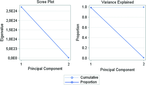
Number of Principal Component versus Eigenvalue of Nominal GDP for the First EU Member Countries (except Germany). Data period from 1967 to 2015.
Source Own processing base on OECD data
First two principal components of Nominal GDP for the First EU Member Countries (except Germany). Data period from 1967 to 2015
Country | PC1 | PC2 |
|---|---|---|
AUT | 0.084 | 0.055 |
BEL | 0.099 | 0.069 |
DNK | 0.066 | 0.032 |
FIN | 0.0524 | 0.0302 |
FRA | 0.5447 | 0.4169 |
GRC | 0.0588 | 0.0343 |
IRL | 0.055 | −0.085 |
ITA | 0.4442 | 0.3649 |
LUX | 0.0117 | −0.001 |
NLD | 0.174 | 0.0651 |
PRT | 0.0505 | 0.0065 |
ESP | 0.3014 | 0.1629 |
SWE | 0.1 | 0.0554 |
UK | 0.5845 | −0.801 |
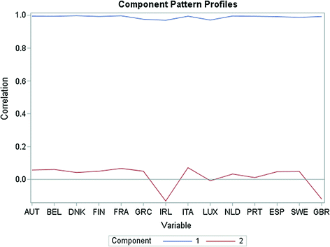
Component Pattern Profiles of Nominal GDP for the First EU Member Countries (except Germany). Data period from 1967 to 2015.
Source Own processing base on OECD data
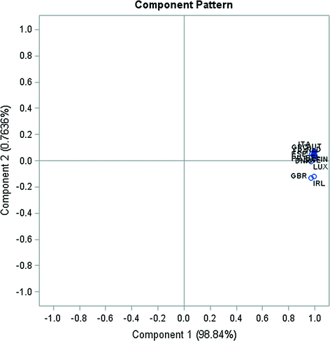
Component Pattern of Nominal GDP for the First EU Member Countries (except Germany). Data period from 1967 to 2015.
Source Own processing base on OECD data
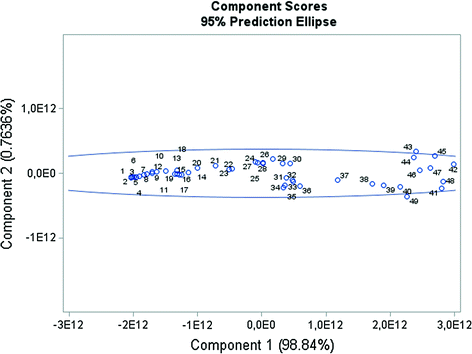
Component Scores of Nominal GDP for the First EU Member Countries (except Germany). Data period from 1967 to 2015.
Source Own processing base on OECD data
Linear regression results of Nominal GDP for France. Data period from 1967 to 2015
Analysis of variance | |||||
|---|---|---|---|---|---|
Source | DF | Sum of square | Mean square | F value | Pr > F |
Model | 2 | 3.89E+25 | 1.94E+25 | 15,124 | <0.0001 |
Error | 46 | 5.91E+22 | 1.28E+21 | ||
Corrected | 48 | ||||
Parameter estimates | |||||
|---|---|---|---|---|---|
Variable | DF | Parameter estimate | Standard error | t value | Pr > |t| |
Intercept | 1 | 1.28E+12 | 5.12E+09 | 250.04 | <0.0001 |
PC1 | 1 | 8.98E+11 | 5.17E+09 | 173.53 | <0.0001 |
PC1 | 1 | 6.04E+10 | 5.17E+09 | 11.67 | <0.0001 |
Linear regression results of Nominal GDP for Luxembourg. Data period from 1967 to 2015
Analysis of variance | |||||
|---|---|---|---|---|---|
Source | DF | Sum of square | Mean square | F value | Pr > F |
Model | 2 | 1.80E+22 | 8.98E+21 | 379.43 | <0.0001 |
Error | 46 | 1.09E+21 | 2.37E+19 | ||
Corrected | 48 | 1.90E+22 | |||
Parameter estimates | |||||
|---|---|---|---|---|---|
Variable | DF | Parameter estimate | Standard error | t value | Pr > |t| |
Intercept | 1 | 2.00E+10 | 6.9E+08 | 29.37 | <0.0001 |
PC1 | 1 | 1.9E+10 | 7.00E+08 | 27.55 | <0.0001 |
PC1 | 1 | −2.00E+08 | 7.00E+08 | −0.23 | 0.8193 |
There is a positive linear relationship between the French GDP and the principal components as the estimated regression coefficients acquire positive values. If the value of the first principal component increases by one unit, the GDP in France will increase by 8.98E+11 USD on average.
Simultaneously the value of the second principal component remains unchanged. Based on the regression results, both regression coefficients are statistically significant, indicating a significant impact of the principal components on the GDP in France. Additionally, the model meets the iid. assumptions. It explains 99.85% of the French GDP. 0.15% of the country’s variability in the GDP is due to other factors than the development of the GDP in the analyzed countries.
From the regression model we received an important information, which is presented in the Table 5. If the GDP of the countries represented by the second principal component increases by one unit, then the GDP of Luxembourg will decrease on average by −2E+08 USD. Additionally, only the first principal component has a statistically significant impact on Luxembourg’s GDP. While the model as a whole is statistically significant, the residuals do not meet the assumptions of normal distribution. The residuals have a systematic tendency. The Durbin Watson’s statistic equals to 0.079, showing a positive autocorrelation
4.2 Nominal GDP During the Period from 1995 to 2015
Descriptive Statistics Nominal GDP of Nominal GDP for all EU Member Countries. Data period from 1995 to 2015
Country | Mean | Standard deviation | Country | Mean | Standard deviation |
|---|---|---|---|---|---|
AUT | 3.15E+11 | 9.14E+10 | ITA | 1.73E+12 | 4.44E+11 |
BEL | 3.84E+11 | 1.13E+11 | LVA | 1.83E+10 | 1.04E+10 |
BGR | 3.30E+10 | 1.87E+10 | LTU | 2.71E+10 | 1.51E+10 |
HRV | 4.28E+10 | 1.70E+10 | LUX | 3.91E+10 | 1.67E+10 |
CYP | 1.79E+10 | 6.89E+09 | MLT | 6.68E+09 | 2.53E+09 |
CZE | 1.39E+11 | 6.72E+10 | NLD | 6.57E+11 | 1.97E+11 |
DNK | 2.56E+11 | 7.21E+10 | POL | 3.31E+11 | 1.56E+11 |
EST | 1.44E+10 | 8.18E+09 | PRT | 1.83E+11 | 5.28E+10 |
FIN | 1.99E+11 | 6.04E+10 | ROM | 1.10E+11 | 6.82E+10 |
FRA | 2.14E+12 | 5.83E+11 | SVK | 6.27E+10 | 3.01E+10 |
DEU | 2.92E+12 | 6.67E+11 | SVN | 3.58E+10 | 1.28E+10 |
GRC | 2.19E+11 | 7.30E+10 | ESP | 1.06E+12 | 3.81E+11 |
HUN | 9.72E+10 | 4.03E+10 | SWE | 3.96E+11 | 1.23E+11 |
IRL | 1.81E+11 | 7.53E+10 | UK | 2.22E+12 | 5.80E+11 |
Eigenvalues of the Covariance Matrix of Nominal GDP for all EU Member Countries. Data period from 1995 to 2015
Eigenvalue | Difference | Proportion | Cumulative | |
|---|---|---|---|---|
1 | 1.52E+24 | 1.47E+24 | 0.9541 | 0.9541 |
2 | 5.15E+22 | 0.0322 | 0.9863 |
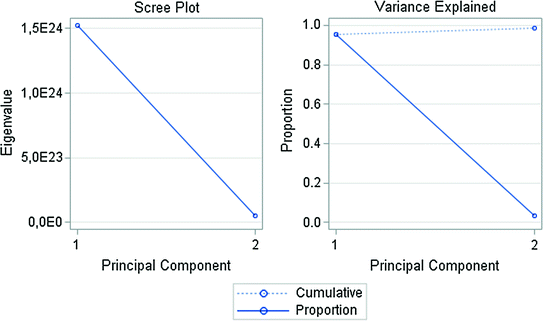
Number of Principal Component versus Eigenvalue of Nominal GDP for all EU Member Countries. Data period from 1995 to 2015.
Source Own processing base on OECD data
First two principal components of Nominal GDP for all EU Member Countries. Data period from 1995 to 2015
Country | PC1 | PC2 |
|---|---|---|
AUT | 0.0734 | −0.0438 |
BEL | 0.0908 | −0.0495 |
BGR | 0.0148 | −0.0055 |
HRV | 0.0136 | 0.0000 |
CYP | 0.0054 | −0.001 |
CZE | 0.0535 | −0.0141 |
DNK | 0.0583 | −0.0157 |
EST | 0.0065 | 0.0017 |
FIN | 0.0488 | −0.0046 |
FRA | 0.4708 | −0.1899 |
GER | 0.5282 | −0.5304 |
GRC | 0.0527 | 0.0163 |
HUN | 0.0322 | 0.0183 |
IRL | 0.0581 | 0.0869 |
ITA | 0.3544 | 0.0128 |
LVA | 0.0083 | 0.0026 |
LTU | 0.012 | 0.0023 |
LUX | 0.0131 | −0.0023 |
MLT | 0.002 | 0.0001 |
NLD | 0.1591 | −0.0197 |
POL | 0.122 | −0.0305 |
PRT | 0.042 | 0.0084 |
ROM | 0.0541 | −0.0096 |
SVK | 0.0241 | −0.0001 |
SVN | 0.0103 | −0.0011 |
ESP | 0.303 | 0.0541 |
SWE | 0.0967 | −0.0264 |
UK | 0.4435 | 0.815 |
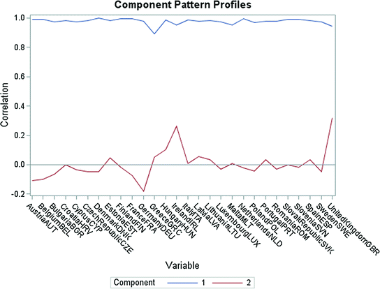
Component Pattern Profiles of Nominal GDP for all EU Member Countries. Data period from 1995 to 2015.
Source Own processing base on OECD data
4.3 Inflation During the Period from 1967 to 2015
Descriptive Statistics of CPI for the selected EU Member Countries. Data period from 1967 to 2015
Country | Mean | Standard deviation |
|---|---|---|
AUT | 3.37 | 2.11 |
BEL | 3.73 | 2.92 |
CYP | 4.16 | 3.32 |
DNK | 4.76 | 3.69 |
FIN | 4.96 | 4.52 |
FRA | 4.48 | 3.97 |
GRC | 9.61 | 8.14 |
IRL | 6.01 | 5.91 |
ITA | 6.43 | 5.84 |
LUX | 3.6 | 2.68 |
MLT | 3.27 | 3.18 |
NLD | 3.47 | 2.61 |
PRT | 9.4 | 8.56 |
ESP | 6.94 | 5.79 |
SWE | 4.62 | 3.95 |
Eigenvalues of the covariance matrix of CPI for the selected EU Member Countries. Data period from 1967 to 2015
Eigenvalue | Difference | Proportion | Cumulative | |
|---|---|---|---|---|
1 | 285.7150 | 252.7744 | 0.8036 | 0.8036 |
2 | 32.9406 | 18.9576 | 0.0926 | 0.8962 |
3 | 13.9830 | 7.4931 | 0.0393 | 0.9355 |
4 | 6.4898 | 0.0183 | 0.9538 |
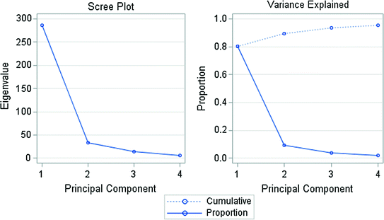
Number of Principal Component versus Eigenvalue of CPI for the selected EU Member Countries. Data period from 1967 to 2015.
Source Own processing base on OECD data
The first principal component represents the most the southern countries of the EU (Portugal, Greece, Italy and Spain) as the first eigenvector has the highest positive loadings on these countries.
The second eigenvector acquires the highest positive loadings on the variable Italy and the lowest loadings on Greece.
The third principal component supremely reflects the inflation in Malta, Greece and Cyprus.
The fourth principal component represents the following countries as the fourth eigenvector acquires the highest positive loadings on Belgium and Luxembourg as well as high negative loadings on Spain and Malta.
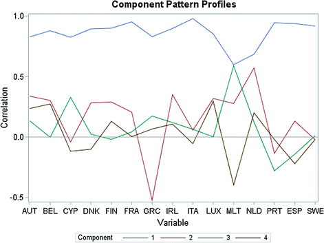
Component Pattern Profiles of CPI for the selected EU Member Countries. Data period from 1967 to 2015.
Source Own processing base on OECD data
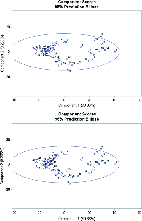
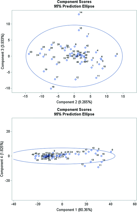
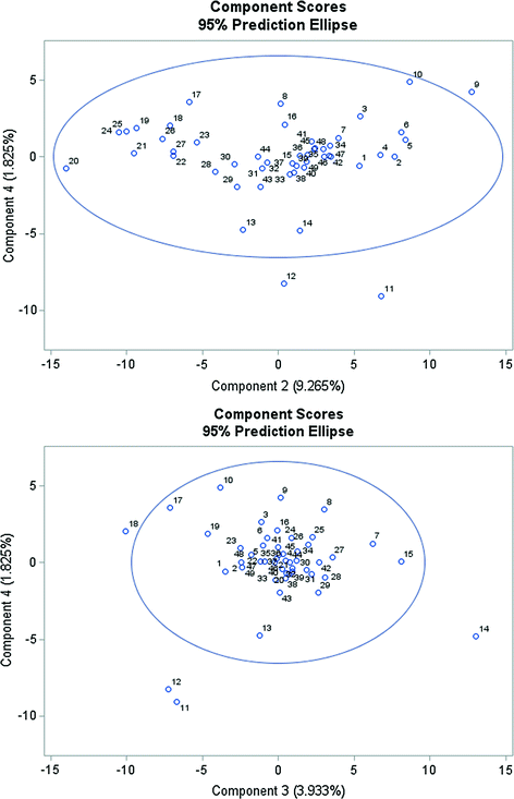
Component Scores with Prediction Ellipse of CPI for the selected EU Member Countries. Data period from 1967 to 2015.
Source Own processing base on OECD data
Linear regression results of CPI for France. Data period from 1967 to 2015
Analysis of variance | |||||
|---|---|---|---|---|---|
Source | DF | Sum of square | Mean square | F value | Pr > F |
Model | 4 | 718.8818 | 179.7204 | 220.31 | <0.0001 |
Error | 44 | 35.8939 | 0.8158 | ||
Corrected Total | 48 | 754.7756 | |||
Parameter estimates | |||||
|---|---|---|---|---|---|
Variable | DF | Parameter estimate | Standard error | t value | Pr > |t| |
Intercept | 1 | 4.4789 | 0.1290 | 34.71 | <0.0001 |
PC1 | 1 | 0.2236 | 0.0077 | 28.99 | <0.0001 |
PC2 | 1 | 0.1424 | 0.0227 | 6.27 | <0.0001 |
PC3 | 1 | 0.0451 | 0.0349 | 1.29 | 0.2028 |
PC4 | 1 | 0.0059 | 0.0512 | 0.12 | 0.9087 |
Linear regression results of CPI for Luxembourg. Data period from 1967 to 2015
Analysis of variance | |||||
|---|---|---|---|---|---|
Source | DF | Sum of square | Mean square | F value | Pr > F |
Model | 4 | 316.88551 | 79.22138 | 121.21 | <0.0001 |
Error | 44 | 28.75891 | 0.65361 | ||
Corrected Total | 48 | 345.64442 | |||
Parameter estimates | |||||
|---|---|---|---|---|---|
Variable | DF | Parameter estimate | Standard error | t value | Pr > |t| |
Intercept | 1 | 3.59736 | 0.11549 | 31.15 | <0.0001 |
PC1 | 1 | 0.13541 | 0.00690 | 19.61 | <0.0001 |
PC2 | 1 | 0.14903 | 0.02033 | 7.33 | <0.0001 |
PC3 | 1 | 0.00089646 | 0.03121 | 0.03 | 0.9772 |
PC4 | 1 | 0.31193 | 0.04581 | 6.81 | <0.0001 |
From the prediction of Luxembourg’s inflation, it is obvious that the CPI index will increase predominantly, if the value of the fourth principal component increases by one unit. Furthermore, the inflation in Luxembourg will increase the least, if the value of the third principal component increases by one unit. The previous facts indicate that an increase in all the principal components causes likewise an increase in the average rate of inflation in the country. Each country included in the analysis affected Luxembourg’s inflation adversely. We can state that the changes in the inflation rates of the countries initiate an increase in the average inflation of Luxembourg. Between the CPI index of the country and the principal components exist a positive linear relationship as the estimations of the regression coefficients are also positive. The results from the table demonstrate the statistical significance of the first, second and fourth principal component. In addition, the model is significant, explaining 91.68% of the overall variability of the data and meets the iid. assumptions too.
According to the values of the Adj. R-Square the model for France is better, while it explains 94.81% of the variability in the input data compared to the model for Luxembourg, where 90.92% of the variability is interpreted.
4.4 Inflation During the Period from 1994 to 2015
Descriptive Statistics of CPI for the all EU Member Countries. Data period from 1994 to 2015
Country | Mean | Standard deviation | Country | Mean | Standard deviation |
|---|---|---|---|---|---|
AUT | 1.9 | 0.78 | ITA | 2.29 | 1.22 |
BEL | 1.88 | 1.04 | LVA | 7.22 | 9.02 |
BGR | 65.28 | 224.16 | LTU | 8.64 | 17.01 |
HRV | 7.73 | 22.27 | LUX | 1.97 | 0.9 |
CYP | 2.26 | 1.77 | MLT | 2.39 | 1.04 |
CZE | 3.91 | 3.4 | NLD | 2.02 | 0.81 |
DNK | 1.96 | 0.74 | POL | 7.34 | 9.13 |
EST | 8.13 | 11.31 | PRT | 2.45 | 1.49 |
FIN | 1.53 | 1.13 | ROM | 29.58 | 41.42 |
FRA | 1.46 | 0.73 | SVK | 5.31 | 3.87 |
DEU | 1.5 | 0.67 | SVN | 5.61 | 4.98 |
GRC | 3.55 | 3.05 | ESP | 2.59 | 1.46 |
HUN | 8.65 | 7.53 | SWE | 1.17 | 1.14 |
IRL | 2.15 | 2.28 | UK | 2.04 | 0.99 |
Eigenvalues of the covariance matrix of CPI for the all EU Member Countries. Data period from 1994 to 2015
Eigenvalue | Difference | Proportion | Cumulative | |
|---|---|---|---|---|
1 | 51230.7264 | 49612.4973 | 0.9633 | 0.9633 |
2 | 1618.2291 | 1433.8253 | 0.0304 | 0.9937 |
3 | 184.4037 | 0.0035 | 0.9972 |
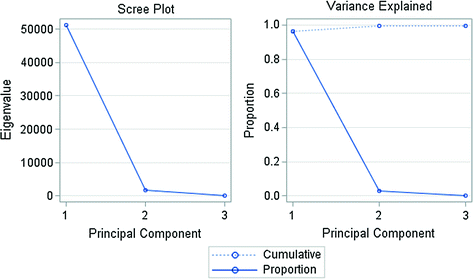
Number of Principal Component versus Eigenvalue of CPI for the all EU Member Countries. Data period from 1994 to 2015.
Source Own processing base on OECD data

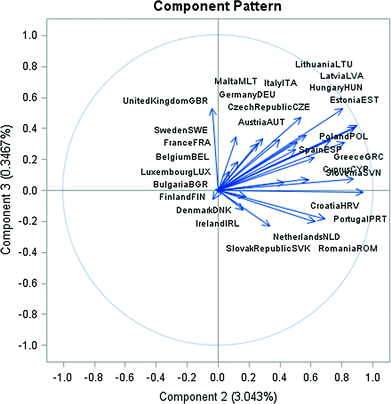
Pairwise Component Pattern of CPI for the all EU Member Countries. Data period from 1994 to 2015.
Source Own processing base on OECD data
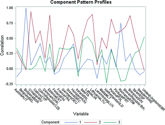
Component Pattern Profiles of CPI for the all EU Member Countries. Data period from 1994 to 2015.
Source Own processing base on OECD data
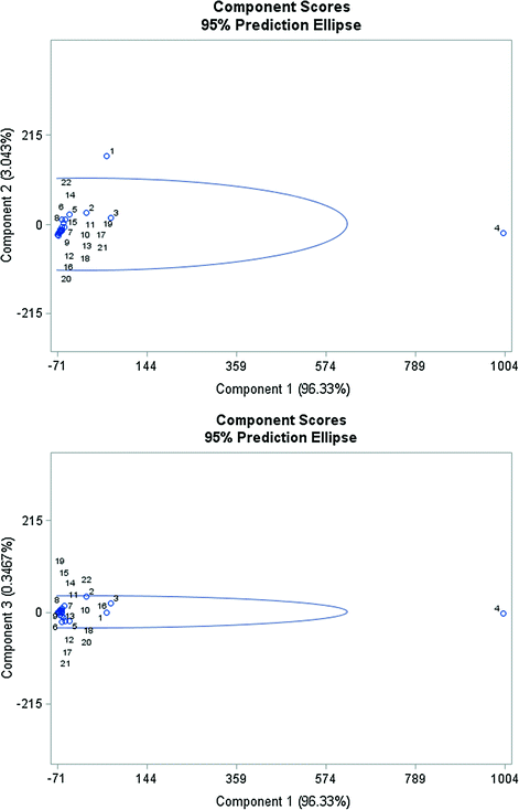
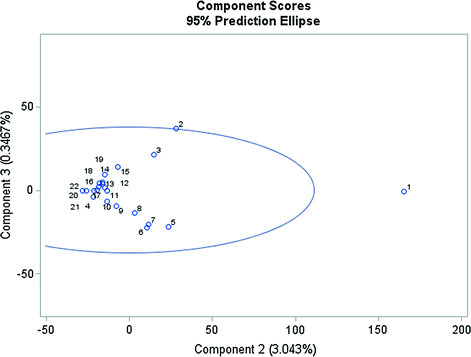
Component Scores of CPI for the all EU Member Countries. Data period from 1994 to 2015.
Source Own processing base on OECD data
The interdependence between the analyzed countries and the principal components can be seen on the Fig. 12. We found that there is either a strong or a moderate correlation between the second component and the countries.
Figure 13 displays components scores and points out the potential outlying years, which are 1994 and 1997. Behind this result is the crisis in Bulgaria and the high rates of inflation in Croatia and Romania at the end of the past century. The countries in central Europe during their economic transformation had high unstable levels of inflation.
5 Conclusion
The main objective of this chapter was to investigate the changes in the inflation and the GDP in the European Union. We analyzed the data over two periods, between 1967–2015 and 1994–2015. We found the main differences among the countries that took place during the analyzed periods.
In the first subchapter we demonstrated the definitions of inflation and the GDP as well as their characteristics. The chapter also contains the possible impacts of inflation on an economy. Additionally, we focused on the principal component analysis. This statistical method enables us to reduce the dimensions of multidimensional data. After obtaining the results from the PCA analysis we determined an adequate number of principal components to represent the countries’ inflation and GDP. We studied whether there exists one principal component that represents most of the countries.
The analysis of inflation during the period from 1994 to 2015 revealed that Austria, Belgium, Cyprus, Denmark, Finland, France, Greece, Ireland, Italy, Luxembourg, Malta, Netherlands, Portugal, Spain and Sweden had lower average inflation and standard deviation in contrary to the analysis over a longer period (1967–2015). The reason behind this could be that the countries, who introduced the euro as their official currency had to meet the Maastricht convergence criteria to be able to entry the euro area and subsequently the common monetary policy.
During the period which stems from 1967 to 2015 we found one principal component explaining 80.36% of the variability in the inflation. This suggests that the inflation in the original countries together with the countries that joined the EU before 1995 was more diverse. These countries formed a more independent system, as we needed four principal components to represent 95.38% of the variability in the data. After comparing the results of the long term (1967–2015) with the shorter-term analyses (1994–2015) we pointed out the dependence of the socialist regime’s succession states from the countries of Western Europe. In the first analysis (1994–2015), the first principal component explained more variability in the data than in the second one (1967–2015).
In the case of GDP both analyses indicate that only one principal component is needed to explain more than 95% of the overall variability in the data. This implies that in the EU there is a strong interdependence between the countries. The first principal component maintained the greatest variability of the original data. Additionally, this principal component the most reflected the GDP in France and the United Kingdom.
The composition of the first principal component was not the same in the two analyses, even though in both the southern countries were dominant in the first principal component. In the longer period the first principal component reflects Italy’s and some of the southern countries’ (Portugal, Greece, Spain) inflation who entered the EU before 1980s. According to the values of the first eigenvector, in the shorter period (1994–2015) a former socialist country, Bulgaria became prevailing in the first principal component. In addition, the PCA results revealed a few problematic years, the hyperinflations in Bulgaria and Yugoslavia in the last century and the global economic and financial crisis in 2009.
In the practical part we explained in more detail the relationship between the principal components, which represent the analyzed countries’ inflation/GDP, and France and Luxembourg. From the conclusions of each regression analysis for inflation it was clear that between the principal components and the two countries is a strong linear relationship. Both models explained more than 90% of the changes in the inflation of these countries. The variability in their price growth was caused by fluctuations of inflation in the countries that joined the EU earlier. The remaining variability may had been caused by various other factors, for example by the changes in fiscal policy, unemployment rates, tax policy or financial market regulations.
The results of the regression analysis of Luxembourg’s GDP revealed that, not all the assumptions about the random error component were met. The residuals did not have a normal probability distribution and had a systematic tendency. In contrary, the scattering analyses suggested that each of the regression model is statistically significant. The slope coefficients were likewise statistically significant.
Based on the values of the Adj. R squares the regression models for France are better as they explain more variability in the countries’ data.
The established regression models provide several viewpoints that can be considered during the monetary and fiscal policy implementations. With relatively high accuracy they can be also applied to predict the GDP in France and Luxembourg.