Appendix B

Details of AFNS Restrictions

Here we provide details of the AFNS restrictions on A₀(3), as calculated using the theory of affine-invariant transformations.

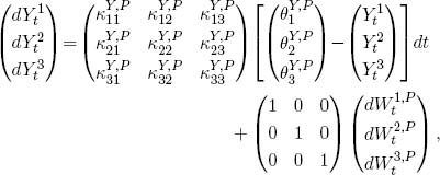
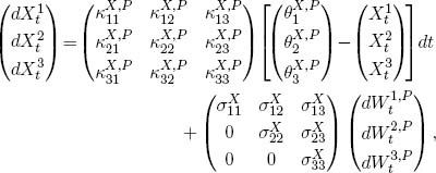
Derivation of the AFNS restrictions imposed on the canonical representation of the A₀(3) class starts with an arbitrary affine diffusion process represented by

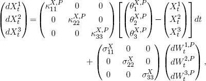
Now consider the affine transformation τ_Y: AY_t + η, where A is a nonsingular square matrix of the same dimension as Y_t and η is a vector of constants of the same dimension as Y_t. Denote the transformed process by X_t = AY_t + η. By Ito’s lemma it follows that

dX_t = AdY_t

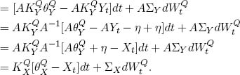
Thus X_t is itself an affine diffusion process with parameters , and Σ_X = AΣ_Y. A similar result holds for the dynamics under the P-measure.

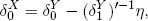
For the short-rate process we have

Thus, defining

and

the short-rate process is unchanged and may be represented either as

or as

Because both Y_t and X_t are affine latent factor processes that deliver the same distribution for the short-rate process r_t, they are equivalent representations of the same fundamental model; hence T_X is called an affine invariant transformation.

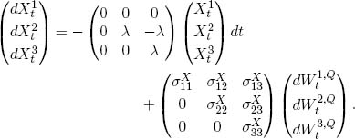
In the canonical representation of the subset of A₀(3) affine term structure models considered here, the Q-dynamics are

the P-dynamics are

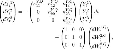
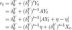
and the instantaneous risk-free rate is

There are 22 parameters in this maximally flexible canonical representation of the A₀(3) class of models, and here we present the parameter restrictions needed to arrive at the affine AFNS models.

B.1 Independent-Factor AFNS

The independent-factor AFNS model has P-dynamics

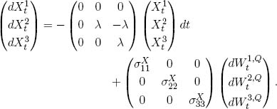
and the Q-dynamics are given by Proposition AFNS as

Finally, the short-rate process is 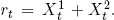This model has a total of 10 parameters; thus 12 parameter restrictions need to be imposed on the canonical A₀(3) model.

It is easy to verify that the affine invariant transformation

τ_A(Y_t)= AY_t + η

will convert the canonical representation into the independent-factor AFNS model, where

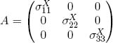
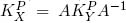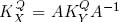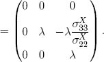
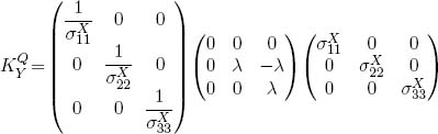
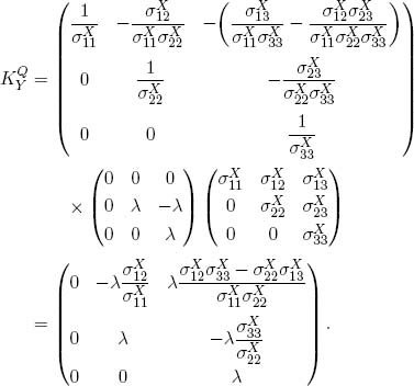
and η = (0 0 0)′. For the mean-reversion matrices, we have , which is equivalent to , and , which is equivalent to . The equivalent mean-reversion matrix under the Q-measure is then

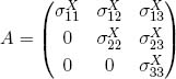
Thus four restrictions need to be imposed on the upper triangular mean-reversion matrix :

Furthermore, notice that the sign of will always be the opposite to that of both and but its absolute size can vary independently of these two parameters. Because , A, and A^–1 are all diagonal matrices, is a diagonal matrix, too. This gives another six restrictions.

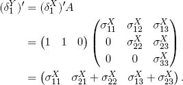
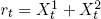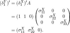
Finally, we can study the factor loadings in the affine function for the short-rate process. In all AFNS models, , which is equivalent to fixing and 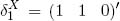. From the relation it follows that

For the constant term we have

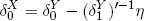
which is equivalent to Thus we have obtained two additional parameter restrictions, and .

B.2 Correlated-Factor AFNS

In the correlated-factor AFNS model, the P-dynamics are

and the Q-dynamics are given by Proposition AFNS as

This model has a total of 19 parameters; thus three parameter restrictions are needed.

It is easy to verify that the affine invariant transformation T_A(Y_t) = AY_t + η will convert the canonical representation into the correlated-factor AFNS model when

and η = (0 0 0)′. For the mean-reversion matrices, we have 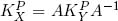, which is equivalent to and 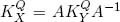, which is equivalent to . The equivalent mean-reversion matrix under the Q-measure is then

Thus two restrictions need to be imposed on the upper triangular mean-reversion matrix and 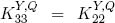. Furthermore, notice that will always have the opposite sign of and , but its absolute size can vary independently of the two other parameters.

Next we study the factor loadings in the affine function for the short-rate process. In the AFNS models, r_t = , which is equivalent to fixing and (1 1 0)′. From the relation , it follows

that

This shows that there are no restrictions on . For the constant term, we have , which is equivalent to . Thus we obtain one additional parameter restriction, . Finally, for the mean-reversion matrix under the P-measure, we have 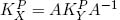, which is equivalent to 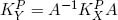. Because is a free 3 × 3 matrix, is also a free 3 × 3 matrix. Thus no restrictions are imposed on the P-dynamics in the equivalent canonical representation of this model.