
Here we begin our journey. We start with static Nelson-Siegel curve fitting in the cross section, but we proceed quickly to dynamic Nelson-Siegel modeling, with all its nuances and opportunities. Among other things, we emphasize the model’s state-space structure, we generalize it to the multicountry context, and we highlight aspects of its use in risk management and forecasting.
As we will see, Nelson-Siegel fits a smooth yield curve to unsmoothed yields. One can arrive at a smooth yield curve in a different way, fitting a smooth discount curve to unsmoothed bond prices and then inferring the implied yield curve. That’s how things developed historically, but there are problems, as discussed in Chapter 1.
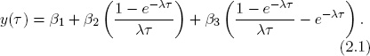
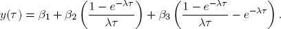
So let us proceed directly to the static Nelson-Siegel representation. At any time, one sees a large set of yields and may want to fit a smooth curve. Nelson and Siegel (1987) begin with a forward rate curve and fit the function
The corresponding static Nelson-Siegel yield curve is
Note well that these are simply functional form suggestions for fitting the cross section of yields.
At first pass, the Nelson-Siegel functional form seems rather arbitrary—a less-than-obvious choice for approximating an arbitrary yield curve. Indeed many other functional forms have been used with some success, perhaps most notably the smoothing splines of Fisher et al. (1995).
But Nelson-Siegel turns out to have some very appealing features. First, it desirably enforces some basic constraints from financial economic theory. For example, the corresponding discount curve satisfies P(0) = 1 and limτ→∞ P(τ) = 0, as appropriate. In addition, the zero-coupon Nelson-Siegel curve satisfies

the instantaneous short rate, and limτ→∞ y(τ) = β1, a constant.
Second, the Nelson-Siegel form provides a parsimonious approximation. Parsimony is desirable because it promotes smoothness (yields tend to be very smooth functions of maturity), it guards against in-sample over-fitting (which is important for producing good forecasts), and it promotes empirically tractable and trustworthy estimation (which is always desirable).
Third, despite its parsimony, the Nelson-Siegel form also provides a flexible approximation. Flexibility is desirable because the yield curve assumes a variety of shapes at different times. Inspection reveals that, depending on the values of the four parameters (β1, β2, β3, λ), the Nelson-Siegel curve can be flat, increasing, or decreasing linearly, increasing or decreasing at an increasing or decreasing rate, U-shaped, or upside-down U-shaped. It can’t have more than one internal optimum, but that constraint is largely nonbinding, as the yield curve tends not to “wiggle” with maturity.
Fourth, from a mathematical approximation-theoretic viewpoint, the Nelson-Siegel form is far from arbitrary. As Nelson and Siegel insightfully note, the forward rate curve corresponding to the yield curve (2.1) is a constant plus a Laguerre function. Laguerre functions are polynomials multiplied by exponential decay terms and are well-known mathematical approximating functions on the domain [0, ∞), which matches the domain for the term structure. Moreover, as has recently been discovered and as we shall discuss later, the desirable approximation-theoretic properties of Nelson-Siegel go well beyond their Laguerre structure.
For all of these reasons, Nelson-Siegel has become very popular for static curve fitting in practice, particularly among financial market practitioners and central banks, as discussed, for example, in Svensson (1995), BIS (2005), Gürkaynak et al. (2007), and Nyholm (2008). Indeed the Board of Governors of the U.S. Federal Reserve System fits and publishes on the Web daily yield Nelson-Siegel curves in real time, as does the European Central Bank.1 We now proceed to dynamize the Nelson-Siegel curve.
Following Diebold and Li (2006), let us now recognize that the Nelson-Siegel parameters must be time-varying if the yield curve is to be time-varying (as it obviously is). This leads to a reversal of the perspective associated with static Nelson-Siegel (2.1), which then produces some key insights.
Consider a cross-sectional environment for fixed t. The Nelson-Siegel model is
This is a cross-sectional linear projection of y(τ) on variables (1, ((1 – e–λτ)/λτ),((1 – e–λτ)/λτ – e–λτ)) with parameters β1, β2, β3.2
Alternatively, consider a time-series environment for fixed τ. The model becomes
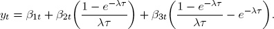
This is a time-series linear projection of yt on variables β1t, β2t, β3t with parameters (1, ((1 – e–λτ)/λτ),((1 – e–λτ)/λτ – e–λτ)).
Hence from a cross-sectional perspective the βs are parameters, but from a time-series perspective the βs are variables. Combining the spatial and temporal perspectives produces the dynamic Nelson-Siegel (DNS) model:
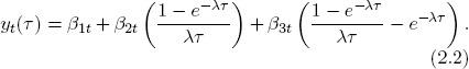
Much of this book is concerned with the DNS model (2.2) and its many variations, extensions, and uses.
Operationally, the DNS model (2.2) is nothing more than the Nelson-Siegel model (2.1) with time-varying parameters. The interpretation, however, is deep: DNS distills the yield curve into three dynamic, latent factors (β1t, β2t, β3t), the dynamics of which determine entirely the dynamics of yt for any τ, and the coefficients (“factor loadings”) of which determine entirely the cross section of y(τ) for any t.
DNS is a leading example of a “dynamic factor model,” in which a high-dimensional set of variables (in this case, the many yields across maturities) is actually driven by much lower-dimensional state dynamics (in this case the three latent yield factors). Dynamic factor models trace to Sargent and Sims (1977) and Geweke (1977).3
Dynamic factor structure is very convenient statistically, as it converts seemingly intractable high-dimensional situations into easily handled low-dimensional situations. Of course, if one simply assumed factor structure but the data did not satisfy it, one would simply have a misspecified model. Fortunately, however, financial asset returns typically do display low-dimensional factor structure. The dozens of bond yields that we see, to take an example close to our interests, clearly are not evolving independently. Instead they tend to move together, not in lockstep of course, as multiple factors are at work, as are idiosyncratic factors, which we will see shortly when we enrich the model. The same is true for stock and foreign exchange markets, as well as for macroeconomic fundamentals, which move together over the business cycle.
Figure 2.1. DNS Factor Loadings. We plot DNS factor loadings as a function of maturity, for λ = 0.0609.
For this reason, factor structure is now central to the theory and practice of financial asset pricing.4
One naturally wants to understand more about the latent factors β1t, β2t, and β3t. Just what are they? What do they do? The answer follows from inspection of the factor loadings, which we plot as a function of maturity in Figure 2.1.
First consider the loading on β2t, (1 – e–λτ)/λτ, a function that starts at 1 but decays monotonically and quickly to 0. Hence it was often called a “short-term factor,” mostly affecting short-term yields.
Next consider the loading on β3t,(1 – e–λτ)/λτ – e–λτ, which starts at 0 (and is thus not short term), increases, and then decays to zero (and thus is not long term). Hence it was often called a “medium-term factor,” mostly affecting medium-term yields.
Finally, consider the loading on β1t, which is constant at 1, and so not decaying to zero in the limit. Hence, unlike the other two factors, it affects long yields and therefore was often called a “long-term factor.”
Thus far we have called the three factors long term, short term, and medium term, in reference to the yield maturities at which they have maximal respective relative impact. Note, however, that they may also be interpreted in terms of their effect on the overall yield curve shape. Immediately, for example, β1t governs the yield curve level: An increase in β1t shifts the curve in parallel fashion, increasing all yields equally, as the loading on β1t is identical at all maturities. Similarly, β2t governs the yield curve slope: An increase in β2t increases short yields substantially (they load heavily on β2t) but leaves long yields unchanged (they load negligibly on β2t).5 Finally, β3t governs the yield curve curvature: An increase in β3t doesn’t change short yields much (they don’t load much on β3t) and doesn’t change long yields much (they too don’t load much on β3t), but it changes medium-maturity yields (they load relatively heavily on β3t).
If β1t governs the level of the yield curve and β2t governs its slope, it is interesting to note, moreover, that the instantaneous yield depends on both the level and slope factors, because yt(0) = β1t + β2t. Several other models have the same implication. In particular, Dai and Singleton (2000) show that the three-factor models of Balduzzi et al. (1996) and Chen (1996) impose the restriction that the instantaneous yield is an affine function of only two of the three state variables, a property shared by the three-factor nonaffine model of Andersen and Lund (1997).
We are now in a position to note that what we have called the “Nelson-Siegel curve” is actually a different factorization than the one originally advocated by Nelson and Siegel (1987), who used
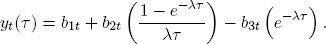
The original Nelson-Siegel yield curve matches ours with b1t = β1t, b2t = β2t + β3t, and b3t = β3t. In the Nelson-Siegel factorization, however, the loadings (1 – e–λτ)/λτ and e–λτ have similar monotonically decreasing shape, which makes it hard to give different interpretations to the different factors b2t and b3t. In our factorization, the loadings have distinctly different shapes and the factors have corresponding distinctly different interpretations as level, slope, and curvature.
Changing to a notation that emphasizes the “level, slope, curvature” interpretation of the DNS factors, we write the DNS model as
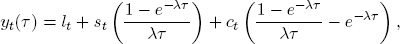
t = 1, … , T, τ = 1, … , N. Following Diebold et al. (2006b), we also now move to a state-space interpretation.
Adding stochastic error terms to the deterministic DNS curve produces the measurement equation, which stochastically relates the set of N yields to the three unobservable yield factors,

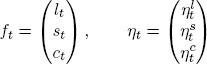
where the variables are
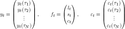
and the parameter matrix is
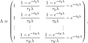
t = 1, … , T. We interpret the stochastic errors εt(τ) as “idiosyncratic,” or maturity-specific, factors. Hence each yield yt(τ) is driven in part by the common factors lt, st and ct (which is why the yield movements cohere in certain ways) and in part by its idiosyncratic factor εt(τ).
Now we need to specify the common factor dynamics, that is, the transition equation. We use a first-order

where the variables are
and the parameter vectors and matrices are
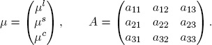
Obviously, µ is the factor mean and A governs the factor dynamics.
The state-space framework is extremely general. For notational convenience we write the state dynamics as first-order in the yield factors, but as is well-known, higher-order dynamics can always be rewritten as a firstorder system. Hence the state-space framework includes as special cases almost any linear dynamics imaginable.6 See Golinski and Zaffaroni (2011) for interesting applications of long-memory ideas in DNS yield curve modeling.
To complete the system we now have only to specify the covariance structure of the measurement and transition disturbances. We make the standard assumptions that the white noise transition and measurement disturbances are orthogonal to each other and to the initial state:
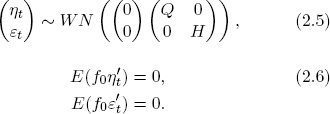
Note that we have not assumed Gaussian measurement and/or transition disturbances. Normality is not required for what follows, although the efficiency properties of various extractions, forecasts, and estimators based on the system (2.3)–(2.6) will differ depending on whether normality is satisfied.
The state-space representation (2.3)–(2.6) is of course not unique. Instead of centering the state vector around a nonzero mean, for example, we could have simply included a constant in either the measurement or transition equation. Such choices are generally inconsequential. However, a deeper issue of identification in factor models typically requires that one normalize either a common factor loading or an idiosyncratic factor variance.
The DNS state-space structure implies that the Kalman filter is immediately applicable for optimal filtering and smoothing of the latent yield factors (in an obvious notation, ft,1:t and ft,1:T), as well as for optimal one-step-ahead or general h-step-ahead prediction of both the yield factors and the observed yields (ft+1,1:t, ft+h,1:t, yt+1,1:t, yt+h,1:t). The optimality of Kalman filter extractions and predictions is in the linear least squares sense. Hence under normality the Kalman filter delivers conditional expectations, whereas more generally it delivers linear projections. These results, and the mechanics of implementing them, are standard.7 Filtering, smoothing, and prediction are of course conditional on a particular set of parameter values. In practice the parameters are unknown and must be estimated, to which we now turn.
Several procedures are available for estimating the DNS model, ranging from a simple two-step procedure, to exact maximum likelihood estimation using the statespace representation in conjunction with the Kalman filter, to Bayesian analysis using Markov-chain Monte Carlo methods. We now introduce them and provide some comparative assessment.
First consider estimation of the static Nelson-Siegel model in the cross section. The four-parameter Nelson-Siegel curve (2.1) is intrinsically nonlinear but may be estimated by iterative numerical minimization of the sum of squares function (nonlinear least squares). Importantly, moreover, note that if λ is known or can be calibrated, estimation involves just trivial linear least squares regression of y(τ) on 1,((1 – e–λτ)/λτ), and ((1 – e–λτ)/λτ – e–λτ).
In practice λ can often be credibly calibrated and treated as known, as follows. Note that λ determines where the loading on the curvature factor ct achieves its maximum. For ct to drive curvature, its loading should be maximal at a medium maturity τm. One can simply choose a reasonable τm and reverse engineer the corresponding λm. Values of m in the range of two or three years are commonly used; for example, Diebold and Li (2006) use m = 30 months. Model fit is typically robust to the precise choice of λ.
The first estimation approach, so-called two-step DNS, was introduced by Diebold and Li (2006). Consider first the case of calibrated λ. In step 1, we fit the static Nelson-Siegel model (2.1) for each period t = 1, … , T by OLS. This yields a three-dimensional time series of estimated factors,  , and a corresponding N-dimensional series of residual pricing errors (“measurement disturbances”),
  .8 The key is that DNS distills an N-dimensional time series of yields into a three-dimensional time series of yield factors,
  .
.
Next, in step 2, we fit a dynamic model to  . An obvious choice is a vector autoregression, but there are many possible variations, some of which we will discuss subsequently. Step 2 yields estimates of dynamic parameters governing the evolution of the yield factors (“transition equation parameters”), as well as estimates of the factor innovations (“transition disturbances”).
The benefits of two-step estimation with calibrated λ (relative to one-step estimation, which we will discuss shortly) are its simplicity, convenience, and numerical stability: Nothing is required but trivial linear regressions. Moreover, one can of course estimate λ as well, if desired, with only a slight increase in complication. The first-step OLS regressions then become four-parameter nonlinear least squares regressions, and the second-step three-dimensional dynamic model for  becomes a four-dimensional dynamic model for
 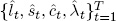 .9 The cost of two-step estimation is its possible statistical suboptimality, insofar as the firststep parameter estimation error is ignored in the second step, which may distort second-step inference.
The second estimation approach, which was introduced by Diebold et al. (2006b), is so-called one-step DNS. The basic insight is that exploitation to the statespace structure of DNS allows one to do all estimation simultaneously.
One-step estimation can be approached and achieved in several ways. On the classical side, exact maximum-likelihood estimation may be done using the Kalman filter, which delivers the innovations needed for evaluation of the Gaussian pseudo likelihood, which can be maximized using traditional (e.g., gradient-based) numerical methods. Alternatively, still using the Kalman filter, one can find the likelihood maximum using dataaugmentation methods such as the expectation maximization (EM) algorithm. Finally, if one is willing and able to specify prior distributions for all coefficients, one can again exploit the state-space structure of DNS to do a full Bayesian analysis.10
As is well-known, running the Kalman filter on the state-space representation of our model (2.3)–(2.4) delivers the one-step-ahead prediction errors with which the Gaussian pseudo likelihood can be evaluated for any parameter configuration. One may then find numerically the parameter configuration that maximizes the likelihood. Traditional gradient-based optimization methods, as used, for example, in Diebold et al. (2006b), are historically the most popular approach, and refinements such as the analytic score functions provided by Koopman and Shephard (1992) can be incorporated to improve performance.
However, the N-yield system (2.3)–(2.6) has many parameters. The measurement equation (2.3) has no parameters with fixed λ, and one parameter with estimated λ. The transition equation (2.4), however, has 12 parameters (three means and nine dynamic parameters). And, crucially, the measurement and transition disturbances have rich variance-covariance structure (2.5). The measurement disturbance covariance matrix has (N2 + N)/2 parameters, and the transition disturbance covariance matrix has six parameters.
This is a large number of parameters to estimate credibly by traditional gradient-based numerical optimization methods. A typical system with 15 yields, for example, has 139 parameters. Even a potentially draconian assumption like diagonal A, Q, and H matrices still leaves N + 10 parameters, a challenging if not absurd situation (and of course one does not generally want to assume such diagonality).
The upshot: QMLE by traditional gradient-based numerical likelihood maximization is often intractable and challenging at best. Another approach replaces traditional gradient-based optimization calculations with a sequence of linear operations that takes one to the same place. The EM algorithm, to which we now turn, does precisely that.
The simple and compelling EM algorithm is tailor-made for state-space models, exploiting the insight that if the parameters are known, then it’s easy to make a good guess of the state sequence, and conversely, if the state sequence is known, then it’s easy to construct a good estimate of the parameters. The EM algorithm converts likelihood maximization into an iterative sequence of state extractions and linear regressions, and it is guaranteed to increase the likelihood at each iteration.11
The intuition of the EM algorithm is strong. Imagine that we somehow know the state vector,  . Then parameter estimation is straightforward; estimation of the measurement equation (2.3) is just estimation of a seemingly unrelated regression system, and estimation of the transition equation (2.4) is just estimation of a first-order vector autoregression, both of which are standard, stable, and fast.
In reality, of course, we don’t know the state vector, but for any given parameter configuration we can extract it optimally using the Kalman filter. (That’s roughly the E step.) Then, conditional on that extracted state vector, we can run the seemingly unrelated regression and vector autoregression above and get new, updated parameter estimates. (That’s roughly the M step.) Then, using the updated parameter estimates we can get an updated state vector extraction, and so forth, continuing iteratively until convergence.
Note that the two-step DNS estimator is very similar to one iteration of EM. In two-step DNS we run one set of regressions (one time) to estimate the state vector, and then conditional on that estimated state vector we run another set of regressions (one time) to estimate the system parameters.
Perhaps surprisingly, although high-dimensional parameter spaces always present challenges, the high-dimensional observed vector of yields also presents problems regardless of the number of underlying parameters, because it makes for slow Kalman filtering and smoothing. Hence slow filtering affects both the gradient-based optimization of section 2.4.3.1 and the EM-based optimization of section 2.4.3.2.
Jungbacker and Koopman (2008), however, show how to achieve fast filtering. They show that dynamic factor models may generally be transformed such that the observed vector is of the same dimension as the state vector. Their approach, together with the efficient multivariate filtering methods of Koopman and Durbin (2000) and the earlier-mentioned analytic score function of Koopman and Shephard (1992), helps deliver practical gradient-based numerical Gaussian QMLE.
Alternatively, as discussed earlier, one can dispense with gradient methods and use EM instead. The Jungbacker and Koopman (2008) and Koopman and Durbin (2000) results are equally useful in that context, however, because it still requires many runs of the Kalman filter.
Finally, one can often blend the methods productively. Two-step DNS, for example, may provide quick and accurate startup values for EM iteration. The EM algorithm, moreover, typically gets close to an optimum very quickly but is ultimately slow to reach full convergence.12 Hence one may then switch to a gradient-based method, which can quickly move to an optimum when given highly accurate startup values from EM.
Optimization in high-dimensional spaces is always a challenging problem. Some of the methods or combinations of methods discussed thus far may confront that problem better than others, but all must nevertheless grapple with it.
Moving to a Bayesian approach may therefore be helpful, because it replaces optimization with averaging in the estimation of moments (e.g., posterior means). Averaging is mathematically easier than optimization.13
Quite apart from the pragmatic motivation above, Bayesian analysis of DNS may also be intrinsically appealing for the usual reasons (see, for example, Koop (2003)) as long as one is willing and able to specify a credible prior and likelihood. The multimove Gibbs sampler of Carter and Kohn (1994) facilitates simple Bayesian analysis of state-space models such as DNS.14
In addition, Bayesian analysis may be especially appealing in the DNS context because there is a potentially natural shrinkage direction (i.e., a natural prior mean), corresponding to the restrictions associated with the absence of arbitrage possibilities. We shall subsequently have much to say about absence of arbitrage, what it implies in the DNS context, and whether its strict imposition is desirable. Bayesian shrinkage estimation is potentially appealing because it blends prior and data information, coaxing but not forcing the MLE toward the prior mean, with the exact amount depending on prior precision versus likelihood curvature. In any event, if one is going to shrink the maximum-likelihood estimates in one direction or another, a natural shrinkage direction—and one clearly motivated by financial economic theory—would appear to be toward no-arbitrage.
In our view, there is no doubt that the state-space framework is a powerful and productive way to conceptualize the structure and estimation of DNS. There is also little doubt that the one-step estimation afforded by the state-space framework is superior to two-step estimation in principle.
We conjecture, however, that little is lost in practice by using two-step estimation, because there is typically enough cross-sectional variation such that  , ŝt, and ĉt are estimated very precisely at each time t. Moreover, in applications we have found that gradient-based one-step estimation is frequently intractable or incompletely trustworthy. In particular, if forced to choose between two-step and traditional gradient-based one-step estimation procedures, we would lean toward the two-step method. When traditional one-step converges, two-step nevertheless tends to match closely, but one-step doesn’t always converge in a trustworthy fashion, whereas two-step is always simple and trustworthy.15
The EM and Bayesian one-step methods that we sketched above, however, are in certain respects much more sophisticated and more numerically stable than traditional gradient-based one-step methods. Bayesian Markov-chain Monte Carlo methods are, after all, now frequently and successfully employed in modeling environments with many hundreds of parameters, and there is no obvious reason why DNS should be an exception. Hence it will be interesting to see how the literature develops as experience accumulates, and which estimation approach is ultimately preferred.
The state-space structure of DNS makes it easy to generalize to incorporate a layered, hierarchical structure. This is useful for modeling sets of yield curves, which arise naturally in multicountry analyses in which country yields can depend on country factors, and country factors can depend on global factors, as in Diebold et al. (2008).16
Imagine a set of “global yields,” each of which depends on latent global common level, slope, and curvature factors and a global idiosyncratic factor,
where the Yt(τ) are global yields, Lt, St, and Ct are global common factors, and Et is a global idiosyncratic factor.
We endow the global common factors with simple autoregressive dynamics,

where  ,
,  , and
, and  are global state transition shocks, or, in a more concise notation that we will use later,

where Ft = (Lt, St, Ct)′ and 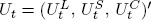 .
.
One might wonder what, precisely, are “global yields,” and from where we obtain data for them. It turns out that we don’t need data for them, as we will soon show.
In a multicountry layered factor framework, each country’s yield curve remains characterized as in standard DNS,
where lit, sit, and cit are latent level, slope, and curvature country common factors and εit is a country idiosyncratic factor.17
Now, however, the country common factors lit, sit, and cit load on the global common factors Lt, St, and Ct, respectively:

where  ,
,  , and
, and  are constant terms,
  ,
,  , and
, and  are loadings on global common factors, and
  ,
,  , and
, and  are zero-mean stochastic disturbances.
Stacking across maturities and countries, the transition equation remains (2.9), which we repeat for convenience:

The measurement equation (in an obvious notation) is

where yt contains yields (for all countries and maturities), Λ contains the DNS factor loadings (for all maturities), A contains the intercepts in the equations relating country factors to global factors (for all countries and country factors), B contains the slopes in the equations relating country factors to global factors (for all countries and country factors), ηt contains the stochastic shocks in the equations relating country factors to global factors (for all countries and country factors), and εt contains the yield curve stochastic shocks (for all countries and maturities).
Note that we do not require observation of global yields or global yield factors. Global yields Yt(τ) do not appear at all in the state-space representation, the measurement equation of which instead relates observed country yields to the latent global yield factors Lt, St, and Ct, which appear in the state vector. Once the model is estimated, Lt, St, and Ct can be extracted using the Kalman smoother.
A variety of assumptions are possible regarding the serial correlation and cross-correlation structures of the various shocks (and indeed whether and where the shocks appear). Thus far, we have been deliberately vague to avoid locking ourselves into any particular special case. Simplest is to assume that all shocks are white noise, orthogonal to all other shocks at all leads and lags. But one could easily imagine wanting more flexibility, for example, through serially correlated η shocks, which would allow for country common factor dynamics other than those inherited from the global common factors.
Many approaches to identification are also possible. The issue of identifying restrictions is related to the issue of stochastic assumptions. In many cases the traditional approaches of normalizing selected factor loadings and/or variances will suffice, but the details necessarily depend on the specific model adopted.
Quite apart from technical issues of statistical flexibility and parameter identification, interesting economic extensions of the basic model (2.7)–(2.13) are also possible. For example, one could allow for more layers in the hierarchical factor structure. Country factors, for example, might depend on regional factors (e.g., Europe, Asia), which then might depend on global factors.
The standard bond portfolio risk measure, duration, measures the sensitivity of bond portfolio value to interest rate changes. In multifactor environments, however, the well-known Macaulay duration (e.g., Campbell et al. (1997)) is an inadequate measure of bond portfolio risk, because it accounts only for level shifts in the yield curve. That is, it is effectively based on a one-factor model.
Hence authors such as Chambers et al. (1988), Willner (1996) and Diebold et al. (2006a) propose generalized duration measures, or so-called duration vectors.18 Each element of a duration vector captures bond price sensitivity to a particular factor. The three-factor DNS model immediately suggests generalized duration components corresponding not only to level, but also to slope and curvature.
In general we can define a bond duration measure as follows. Let the cash flows from the bond be C1,C2, … , CI, and let the associated times to maturity be τ1, τ2, … , τI. Assume also that the zero-coupon yield curve is linear in a set of arbitrary factors. In keeping with our DNS perspective we assume three factors, f1, f2, and f3, but of course more could be added. We write
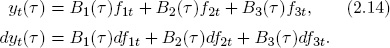
Then, assuming continuous compounding, the price of the bond is
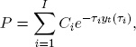
where we discount cash flow Ci using the corresponding zero-coupon yield yt(τi). For an arbitrary yield curve movement, the price change is
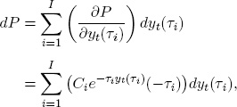
where we have treated yt(τi) as independent variables.
Therefore
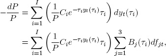
where we have used (2.14) to produce the second equality. Rearranging terms, we can express the percentage change in bond price as a function of changes in the factors

where wi is the weight associated with Ci.
In (2.15), we decomposed the bond price change into changes coming from different risk factors. Hence we can define the duration component associated with each risk factor as

In particular, the duration vector of any coupon bond, based on the three-factor DNS model, is
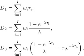
Note that the first element of the duration vector is exactly the traditional Macaulay duration, while the second and third elements capture response to nonlevel (i.e., slope and curvature) shifts.19
Verifying that the elements of the DNS duration vector increase with τ, decrease with the coupon rate, and decrease with the yield to maturity is straightforward. In addition, they have the “portfolio property”: a bond portfolio’s Dj is a weighted average of its component bonds’ Dj’s, where the weights assigned to the component bonds are their shares in portfolio value.
There are by now literally hundreds of DNS applications involving model fitting and forecasting. The original paper of Diebold and Li (2006) finds good fits and forecasts for a certain sample of U.S. government bond yields, but subsequent empirical results of course vary across studies that involve different sample periods, different sets of yields, different countries, and so forth. For example, Mönch (2008) finds that the clear superiority of DNS found in Diebold and Li (2006) is not confirmed on a certain set of subsequent U.S. data, whereas Alper et al. (2007) find good forecasting performance for another country (Turkey). Nevertheless, all told, DNS tends to fit and forecast well, which, combined with its simplicity, is responsible for its popularity. Here we elaborate.
First consider DNS fits. Nelson-Siegel and related three-factor models of level, slope, and curvature have been observed to fit well in the cross section for several decades, from the original work of Nelson and Siegel (1987) through the ongoing fits of Gürkaynak et al. (2007), written to the Web daily by the U.S. Federal Reserve.20
Good cross-sectional fit is not too surprising, because Nelson-Siegel is actually quite a flexible functional form. Nelson-Siegel curves are smooth, and real yield curves tend to be smooth. They can have at most one internal optimum, but that restriction is rarely violated in the data. They can be flat, increasing or decreasing at increasing, decreasing, or constant rates. Of course they don’t fit observed yields exactly, but from a predictive viewpoint that’s natural and desirable, as their tightly parametric structure guards against in-sample overfitting.
Now consider the fit of dynamic Nelson-Siegel. A well-fitting dynamic model of yield curve dynamics must match not only the historical facts concerning the average shape of the yield curve and the variety of shapes assumed at different times, but also the dynamic evolution of those shapes.
For a parsimonious model to accord with all observed shapes and dynamic patterns is not easy, but let us consider some of the most important stylized facts and see whether and how DNS is capable of replicating them:
(1) The average yield curve is increasing and concave.
In our framework, the average yield curve is the yield curve corresponding to the average values of lt, st and ct. It is certainly possible in principle that it may be increasing and concave, depending on the average values of lt, st and ct.
(2) The yield curve takes a variety of shapes, including upward sloping, downward sloping (“inverted”), humped, and inverted humped.
In our framework, the yield curve can assume all of those shapes. Whether and how often it does depends upon the values of, and variation in, lt, st, and ct.
(3) Yield dynamics are highly persistent, and spread dynamics are much less persistent.
In our framework, persistent yield dynamics correspond to strong persistence of lt, as all yields load equally on lt, which is certainly possible. In addition, if yield persistence is largely driven by common dependence on lt, then the lt effect should be eliminated by moving to spreads, which will then be less persistent.
Alternatively, spread dynamics that are less persistent could also be reflected in less persistence of st, as the yield curve slope is closely related to the long–short spread. This behavior is certainly possible in the DNS framework.
The key is to recognize that DNS distills a time series of yield curves into a three-variable time series of yield factors, so that different sorts of factor dynamics produce different sorts of yield curve dynamics.
Now consider DNS forecasts. In the DNS framework, forecasting the yield curve just amounts to forecasting a three-variable time series of factors. An obvious simple choice of model for the factors is a first-order vector autoregression. Beginning with the original paper of Diebold and Li (2006), however, many have noticed that an unrestricted vector autoregression is outperformed by a restricted version with diagonal coefficient matrix and innovation covariance matrix. Such “orthogonal state variables” are motivated by the common empirical finding that the DNS level, slope, and curvature factors are quite close (although of course not identical) to the first three yield principal components, which are orthogonal by construction. Recently some authors even work with theoretical models that force orthogonality, as in Lengwiler and Lenz (2010).
Figure 2.2 provides a good stylized summary of typical DNS forecast performance. For 1-, 6-, and 12-month forecast horizons and a variety of maturities, we show out-of-sample DNS root mean squared forecast error relative to that of a “no-change” (random walk) forecast. Several important results emerge.
First, the one-month DNS forecasts fare no better than no-change forecasts. This is unsurprising insofar as one month is quite a short horizon, at which the yield-factor mean reversion captured by DNS may have insufficient time to operate. To see this, consider, for example, one-minute-ahead yield curve forecasts, in which case “no change” is likely to be unbeatable!
Second, as the horizon lengthens somewhat to 6-month and 12-month, the relative performance of DNS improves dramatically. The intuition is the same: Although “no change” is a good approximation to the optimal forecast at the shortest horizons, it’s a poor forecast at longer horizons, because it fails to capture the mean reversion in yield factors. Hence DNS fails to beat no change at the shortest horizons but beats it soundly at longer horizons. Empirically, it often happens that relative DNS performance is optimized at 6- to 12-month horizons.21
Figure 2.2. Out-of-Sample Forecasting Performance: DNS vs. Random Walk. For three forecast horizons and a variety of maturities, we show out-of-sample DNS root mean squared forecast error relative to that of a “no-change” forecast.
This may be particularly useful, as such horizons correspond to typical holding periods in many asset allocation strategies.
Third, the forecast accuracy gains delivered by DNS tend to come at short and medium maturities. We will have more to say about that in subsequent chapters when we introduce additional yield factors.
In closing, we would like to elaborate on the likely reason for DNS’s forecasting success: DNS imposes a variety of restrictions, which of course degrade in-sample fit, but which may nevertheless be helpful for out-of-sample forecasting. The essence of our approach is intentionally to impose substantial a priori structure, motivated by simplicity, parsimony, and theory, in an explicit attempt to avoid data mining and hence enhance out-of-sample forecasts in the small samples encountered in practice. This includes our use of a tightly parametric model that places strict structure on factor loadings in accordance with simple theoretical desiderata for the discount function, our emphasis on simple univariate modeling of the factors based upon our theoretically derived interpretation of the model as one of approximately orthogonal level, slope, and curvature factors, and our emphasis on the simplest possible orthogonal AR(1) factor dynamics.
1 The FRB and ECB curves are actually based on an extension of Nelson-Siegel introduced in Svensson (1995), which we discuss and extend even further in Chapter 4.
2 For now, assume that λ is known. We will elaborate on λ later.
3 See also Watson and Engle (1983).
4 See, for example, Campbell et al. (1997) and Cochrane (2001).
5 It is interesting to note that some authors, such as Frankel and Lown (1994), define the yield curve slope as yt(0) – yt(∞), which is exactly equal to β2t.
6 One exception—perhaps the only exception of interest—is long-memory dynamics, which do not admit representation with finite-dimensional state. Long-memory processes can, however, be approximated arbitrarily well by sums of simple first-order autoregressions, as shown by Granger (1980).
7 For details see standard texts such as Harvey (1990).
8 Note that because the maturities are not equally spaced, we implicitly weight the most “active” region of the yield curve most heavily when fitting the model, which seems desirable. It would be interesting to explore loss functions that go even further in reflecting such economic considerations, based, for example, on bond portfolio pricing or success of trading rules, such as that done in different but related contexts by Bates (1999) and Fabozzi et al (2005). Thus far, the DNS literature has not pursued that route aggressively.
9 Note that we have thus far considered two rather extreme cases for λ: calibrated and fixed, or estimated and time-varying. One might of course be interested in the intermediate case of λ estimated but fixed. This turns out to be challenging with two-step estimation, but simple with the one-step estimation introduced later.
10 For algorithmic detail regarding Bayesian analysis of state-space models, see, for example, Koop (2003). Here we stress issues and intuition.
11 See Tanner (1993) for a more detailed discussion of EM, related methods, and relevant references. The classic econometric implementation of EM in dynamic factor models is Watson and Engle (1983), and Reis and Watson (2010) provide a recent econometric application in a high-dimensional situation.
12 In the original EM paper, Dempster et al. (1977) show that EM converges at a linear rate, in contrast to the faster quadratic rate achieved by many gradient-based algorithms.
13 Optimization and averaging are of course related, however, as emphasized by Chernozhukov and Hong (2003).
14 See also the exposition and insightful applications in Kim and Nelson (1999).
15 In addition, within the two-step estimation paradigm one could use the methods of Pagan (1984) to formally address the “generated regressor” problem, possibly enhancing the reliability of second-step tandard errors. To the best of our knowledge, the DNS literature thus far has featured neither a comparison of one-step vs. two-step estimation nor a comparison of two-step estimation vs. “generated regressor adjusted” two-step estimation.
16 Similar structures have been used effectively in the macroeconometric literature on global business cycle modeling, including Gregory et al. (1997), Kose et al. (2008), and Aruoba et al. (2011).
17 Note that we have fixed λ over both time and space. It might be interesting to relax that assumption.
18 See also Garbade (1999).
19 DNS-based vector duration, with its good properties asymptotically in τ, contrasts to the closely related polynomial-based vector duration proposed by Chambers et al. (1988), 
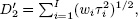 and
and 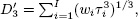 which suffers from the bad properties of polynomials asymptotically in τ.
20 Gürkaynak et al. (2007) actually use a very close four-factor variant of Nelson-Siegel, which we introduce in the next chapter.
21 At extremely long horizons the relative DNS performance again deteriorates, as both forecasts are poor—the no-change forecast is the current yield curve as always, and the DNS forecast is effectively the unconditional mean yield curve.

