Chapter 8

0–1 Knapsack Problems ¹

8.1. General solution principle

This chapter is devoted to obtaining an exact solution, which is both effective and robust, to the knapsack problem with one constraint and n 0–1 variables, which is formulated as follows:

where all the data c = (c_j)_j=1,…,n, a = (a_j)_j=1,…,n and b are assumed to be in , with the standard hypothesis:

which avoids two trivial situations: elimination of the variables x_j such that a_j > b, and an optimal solution with all the variables equal to 1.

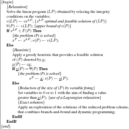
The general solution principle of a linear program with 0–1 variables is applied to the knapsack problem with two fundamental particularities that allow us to obtain an effective and robust method (Figure 8.1):

(i) The algorithms used in the preprocessing phase (relaxation, greedy heuristic, reduction of (P) through variable fixing) are all of linear complexity.

(ii) The exact solution phase (implicit exploration of the set of the solutions of the reduced problem) is carried out by combining a tree search method (branch-andbound) and a dynamic programming method. The effectiveness obtained by algorithmic choices and data structures that favor simplicity and incrementality, is associated with the robustness induced by this hybridization.

Notations

xP	: optimal and feasible solution of (P)
v(P)	: value of (P)
F(P)	: set of the feasible solutions of (P)

Figure 8.1. Exact solution method for the 0–1 knapsack problem

8.2. Relaxation

Solving the linear program associated with (P):

can be carried out by an algorithm of linear time complexity on average by adapting a best elements list search method based on the fast sorting method “Quicksort” [SED 78]. Theorem 8.1 gives the very particular structure of a feasible and optimal solution of (LP).

THEOREM 8.1.– Given a tripartition U,{i}, L of {1, 2,…, n} such that:

(i)

(ii)

a feasible and optimal solution of (LP) is defined as follows:

and:

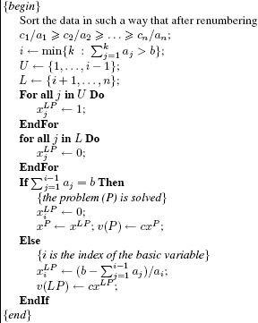
When n is small (for example less than 8 [FAY 79, FAY 82]), it is sufficient to apply a complete sort algorithm of the ratios c_j/a_j to obtain x^LP (see Figure 8.2).

EXAMPLE 8.1.– We consider the following instance with eight variables:

The complete sort of the ratios c_j/a_j:

allows us to conclude that U = {4, 6, 1,7, 2}, i = 8 and L = {3, 5} since:

Figure 8.2. Solving (LP) using a complete sort of the c_j/a_j

and:

In the opposite case, (LP) can and must be solved by an algorithm of linear complexity based on the principle of searching for the k best elements of a list of n elements (given k less than n). This search can be done with a time complexity of O(n) on average by adapting the Quicksort method. The proof of its complexity can be found in [SED 78].

This algorithm is based on the following principle. To determine the k best elements (indexed by U) in a list T of n elements t_j that has an order relationship (k is assumed to be a positive integer less than n), it is sufficient to choose a reference element h in E = {1, 2,…, n} and to create a tripartition E₁, {h}, E₂ of E such that:

Three cases arise:

(i) card(E₁) > k ⇒ the process must be iterated on the elements indexed by E₁;

(ii) card(E₁) + 1 < k ⇒ the process must be iterated on the elements indexed by E₂ in the knowledge that U contains E₁ ∪ {h};

(iii) card(E₁) = k (or card(E₁) + 1 = k respectively), the t_j j ∈ E₁ (or E₁ ∪ {h} respectively) are the best in T.

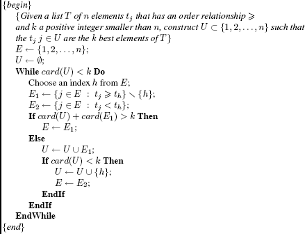
which gives the algorithm in Figure 8.3.

EXAMPLE 8.2.– Search for the six largest elements in the set:

Step1: from E = {1,2,3,4,5,6,7,8,9,10}, we choose for example h = 1. The tripartition (made by an alternate search of values of E that allow us to make only assignments without permuting elements) results in:

which, for greater clarity, corresponds with a permuted set T:

It is certain that {15, 40, 20, 10} corresponds to the four best elements of T. We state U = {8, 5,3, 1}. The process must be iterated on E = E₂ to find the two missing elements.

Step 2: from E = {4,6,7,2,9,10}, we choose h = 4 to give:

which corresponds to a permuted set T:

It is certain that elements {3, 1, 2} do not belong to the six largest elements of T. The process must be iterated on E = E₁.

Step 3: from E = {10, 6, 9}, we choose h = 10 to give:

and therefore the six largest elements of T are:

Figure 8.3. Algorithm of linear complexity for the k best elements of a list of n elements

The principle of adapting the algorithm from Figure 8.3 for solving (LP) is the following [BAL 80, FAY 79, FAY 82]: establishing a feasible optimal solution of (LP) consists of finding the maximum number of the greatest ratios c_j/a_j (j in U) that satisfy condition (ii) of theorem 8.1 (here this number is not known but is given implicitly by relationship (ii)).

Following the example presented for the k best elements of a list (k known), it is sufficient to choose a reference element h from E = {1, 2,…, n}, and to create a tripartition E₁, {h}, E₂ of E such that:

Three cases arise for which debate gives rise to the algorithm shown in Figure 8.4:

(i) the process must be iterated on the elements indexed by E₁;

(ii) the process must be iterated on the elements indexed by E₂ in the knowledge that U contains E₁ ∪ {h};

(iii) if (or respectively), the problem (P) is solved with the variables x_j equal to 1 for every j in E₁ (or E₁ ∪ {h} respectively); in the opposite case (that is ) we have U = E₁, i = h and L = E₂.

COMMENT 8.1.– The choice of the reference element can be made in the same way as for the sorting method Quicksort (the median element among the first , the last , and the median element of the list being considered [FAY 82]), or even by the median algorithm that partitions the list into two sublists of identical size but involves an increase in computation times [LAW 79]. Even if the theoretical complexity in the first case is linear, a third way that has been proven experimentally to be the most effective [BOU 92] consists of choosing as partitioning element an “angular pivot”, that is:

COMMENT 8.2.– In Nagih and Plateau [NAG 00c], we find an adaptation of this principle for solving unconstrained hyperbolic 0–1 programs.

EXAMPLE 8.3.– We go back to the instance with eight variables whose data is:

for which we seek the maximum of the largest elements of the set:

Step1: from E = {1, 2, 3, 4, 5, 6, 7, 8}, we choose, for example, h = 1. The tripartition (made by an alternate search of E that allows us to make only assignments) results in:

which, for greater clarity, corresponds to a permuted set T:

Since σ = a₆ + a₄ + a₁ = 21 < b = 43, it is certain that U contains {6,4,1}, which corresponds to the three best elements {1.85, 2, 1.43} of T. The process must be iterated on E = E₂.

Step 2: from E = {3, 5, 2, 7, 8}, we choose h = 3 to give:

which corresponds to a permuted set T:

Since σ + a₈ + a₇ + a₂ = 45 > b, it is certain that L contains E₂ = {3,5}. The process must therefore be iterated on E = E₁.

Step 3: from E = {8, 7, 2}, we choose h = 8 to give:

Since σ + a₂ + a₇ = 37 < b < σ + a₂ + a₇ + a₈ = 45, we conclude that:

and we find the solution x^LP found with the complete sort algorithm of c_j/a_j.

8.3. Heuristic

The aim is to establish a feasible solution x of (P) and therefore a lower bound v(P) of v(P) using an algorithm of linear time complexity. This greedy heuristic (Figure 8.5) consists of exploiting the order of the data provided by the solution of (LP) to keep the objects of U in the knapsack, eliminate the object i, and fill the knapsack of residual capacity with part of the objects of L.

COMMENT 8.3.– The greedy algorithm proposed by Bourgeois and Plateau [BOU 92], which consists of selecting at each step in L the object with the best ratio c_j/a_j, is the most effective on average.

8.4. Variable fixing

The reduction in the size of (P) exploits its branching into two subproblems with the complementary conditions (x_k = 0) and (x_k = 1), where k ∈ {1,…, n}. Thus, since:

assuming that a lower bound v(P) on v(P) and a relaxation (Relax(P : x_k = ε)) of (P : x_k = ε), ε ∈ {0, 1}, are known, if the relation:

is satisfied, then we must state the inverse condition (x_k = 1 − ε) in the hope of finding a feasible solution of value strictly greater than v(P).

We must therefore consider the problem:

Figure 8.4. Solving (LP) using an algorithm of linear complexity

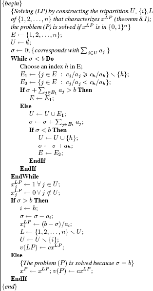
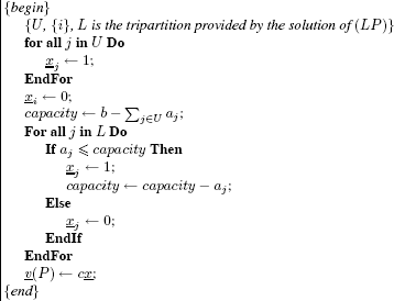
Figure 8.5. Greedy algorithm for the 0–1 knapsack problem

that is the problem (P) whose size is reduced by fixing to 1 − ε the variable x_k (however, the problem (P : x_k = ε) is to be rejected).

We propose applying this scheme to reduce the size of (P) with a linear time complexity. This linear complexity is possible using:

– the greedy algorithm of section 8.3, which establishes a lower bound of v(P); – the Lagrangian dual of (P).

Before detailing the use of the test (*), the following preliminary results are essential.

We recall that (see section 8.2):

where U, {i}, L is the tripartition defined in theorem 8.1. This value can be rewritten in the form:

which is none other than the value of the Lagrangian relaxation of (P):

In this way, since the Lagrangian relaxation of the knapsack satisfies the integrality property, we can conclude that is an optimal multiplier for the Lagrangian dual of the knapsack, that is:

By further observing that:

– on the one hand:

– on the other hand:

we deduce that the test (*) leads us to variable fixings to the values that they have in x^LP, the optimal solution of (LP).

This leads to the following result, which is enhanced by taking into account the integrity of the coefficients of the objective:

THEOREM 8.2.– Given v(P), a lower bound on v(P), if the following relationship is satisfied:

with (k ∈ U and ε = 0) or (k ∈ L and ε = 1), then the variable x_k must be fixed to the value in every solution of value strictly greater than v(P).

By recalling that (LP) may be solved using an algorithm of linear time complexity (section 8.2), and by detecting a feasible solution of (P) using the greedy algorithm from section 8.3, the procedure of fixing variables of U ∪ L can be done in linear time since each test is carried out in O(1).

COMMENT 8.4.– The basic variable x_i cannot be fixed by this process because its reduced cost is zero.

COMMENT 8.5.– The use of linear programming instead of Lagrangian relaxation leads to a gain in the quality of the upper bound but with a time complexity in O(n²). In [FRE 94], the authors proposed a process with two levels that uses linear programming when the test (*) is “almost satisfied” by the Lagrangian relaxation.

EXAMPLE 8.4.– Let there be a knapsack problem with seven 0–1 variables:

whose data is arranged in decreasing order of c_j/a_j; we find successively:

to give the following variable fixings:

and the subproblem:

whose value is clearly equal to 120.

We deduce from this that the value found by the greedy algorithm is optimal and therefore that v(P) = 122 and x^P = (1,1,1,1,0,1,0)^t.

8.5. Dynamic programming

Dynamic programming is a technique much used in combinatorial optimization (for example shortest path problems) and more widely in operations research (see for example [BEL 57, LAU 79, MIT 64]).

In the case of the 0–1 knapsack problem, dynamic programming combined with a branch-and-bound method is a method that has displayed robustness on large classes of instances of the problem (see section 8.6 and [BOU 92, PLA 85]).

Section 8.5.1 presents the principle of solving the 0–1 knapsack problem using dynamic programming. It provides an algorithm of pseudo-polynomial complexity for finding the value of (P), since it takes O(nb), and a linear algorithm in O(n) for establishing an optimal solution of (P).

In fact, effective programs use a relevant management of sets of combinations of objects that allows a gain in memory space and in experimental time complexity. This second version of the dynamic programming algorithm is described in section 8.5.2. It is this version that is combined with branch-and-bound in the hybridization presented in section 8.6.

8.5.1. General principle

We envisage the following n(b + 1) problems:

for l in {1,…, n} and y in {0,…, b}.

For each fixed couple of parameters (l, y), the value of (P_l(y)) is classically denoted by f_l(y) in the literature and is called the knapsack function. Thus we have:

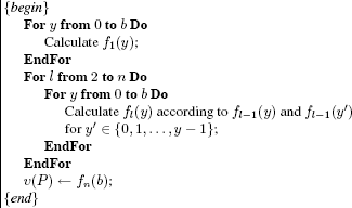
The principle of dynamic programming for the 0–1 knapsack problem is given in Figure 8.6.

More precisely, for a given l 2 (number of variables) and y (right-hand side of the constraint), the dynamic programming algorithm consists of envisaging the branching of the problem (P_l(y)) into two subproblems in which the variable x_l is by turns assumed to be zero and equal to 1:

to give the relation:

Figure 8.6. Principle of dynamic programming for the 0–1 knapsack problem

which compares two values obtained in the preceding iteration (with l − 1 variables), the first at the same level y of the right-hand side of the constraint, the second at the level y − a_l. In effect, since the problem (P_l(y) : x_l = 1) is expressed:

we deduce that v(P_l(y) : x_l = 1) is equal to c_l + f_l−1(y − a_l) if the capacity y is sufficient (that is y a_l) and equal to −∞ in the opposite case (that is the domain is empty).

In this way, we obtain:

Lastly, f₁(y) is calculated as follows ∀ y ∈ {0,…, b}:

Figure 8.7. Dynamic programming for the 0–1 knapsack problem

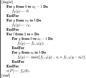
The algorithm given in Figure 8.6 is detailed in full in Figure 8.7. Its time complexity is clearly in O(nb), a complexity said to be pseudo-polynomial since it depends not only on n but also on the right-hand side of the constraint.

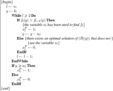
This algorithm only provides the value of the problem (P). To establish an optimal solution x^P of (P) with an additional time complexity O(n), it is sufficient to note that by construction, a solution x^P exists such that ∀ y ∈ {0,…, b}:

and:

for applying the iterative scheme from Figure 8.8.

EXAMPLE 8.5.– For the following 0–1 knapsack problem with four variables:

the table of the values of all the knapsack functions f_l(y), l ∈ {1,…, 4} and y ∈ {0,…, 13} is as follows:

From this we deduce the value of (P):

and the associated optimal solution x^P as follows (see the algorithm from Figure 8.8):

COMMENT 8.6.– The values with a border in the column f₄(y) correspond to the qualitative jumps that will be dealt with exclusively in the algorithm from section 8.5.2.

8.5.2. Managing feasible combinations of objects

The algorithm presented in the previous section assumes a structuring of the data in the form of a table with a memory space in O(nb). It is possible to gain in time and spatial experimental complexities by only managing the set of different feasible combinations of objects (that is that can be put into the knapsack together) that are non-dominated; in other words, it is sufficient to envisage only the set of couples:

that satisfy the following two conditions:

Figure 8.8. Establishing an optimal solution after applying the dynamic programming algorithm

(i) T_J is feasible: ;

(ii) T_J is non-dominated: J′ ⊂ {1,…, n} such that and .

This set is constructed dynamically by considering in turn the first object (that is J ⊆ {1}) then the first two objects (that is J ⊆ {1, 2}), and so on up to considering n objects (that is J ⊆ {1,2,…, n}).

To simplify the notations, we state:

to express T_J in the form (a_J, c_J).

By referring to the numerical illustration in section 8.5.1, we have, for example, T_∅ = (0,0), T_{1} = (a₁,c₁) = (2,10), and T_{1,2} = (a₁ + a₂,c₁ + c₂) = (10,29).

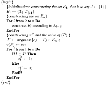
The algorithm consists of envisaging construction of the sets:

firstly for l equal to 1, then equal to 2 and so on up to l equal to n. The value of (P) is situated in the couple T_J* of E_n such that:

Figure 8.9 gives the principle of this algorithm whose dynamic phase (that is the construction of E_l according to E_l−1 ∀ l ∈ {2,…, n}) can be decomposed into two steps as follows:

Step 1: constructing an intermediary set:

which includes all the feasible couples constructed by integrating the object l in the couples of E_l−1 (that is each couple of E′_l is in the form (a_J + a_l, c_J + c_l) with J ⊂ {1,…, l − 1}).

Step 2: merging the sets E_l−1 and E′_l by eliminating the dominated couples, that is by constructing:

We recall that a couple T_J is said to be dominated by a couple T_J′ if the following two conditions are satisfied:

This couple T_J can be eliminated since in the rest of the algorithm all the new couples are constructed by adding combinations of objects in the form (size, value), and evidently the couples (a_J + size, c_J + value) would always be dominated by the couples (a_J′ + size, c_J′ + value) since:

(if it possible to add size to a_J, then, from the construction, it is also possible to add it to a_J′).

In this way, eliminating the dominated couples in every set E_l gives, besides a gain in memory space, an ordering of the set’s elements in a strictly increasing order, that is ∀ J ≠ J′, either a_J < a_J′ and c_J < c_J′, or a_J′ < a_J and c_J′ < c_J.

Figure 8.9. Dynamic programming algorithm with management of the feasible combinations of non-dominated objects

From the construction, this property is also satisfied for sets in the form E′_l.

In practice, following the example of merging sorted lists, with each iteration l, the increasing order of the elements of E_l−1 and of E′_l is naturally maintained; their merging combined with spotting and dynamically eliminating dominated pairs is thus carried out in linear time, that is in O(card(E_l−1 ∪ E′_l)).

Furthermore, by managing the elements of each set E_l in increasing order, the optimal couple that allows us to define the value of (P) and the associated optimal solution is detected in O(1) since it is the last element of E_n.

COMMENT 8.7.– It is possible to deduce a solution and the value from the set E_n (with a time complexity O(card(E_n))) of every problem in the form:

with y ∈ {0, 1,…, b−1},bydetectingthecoupleT_J*(y) such that a_J∗(y) = max{a_J : a_J y}, which allows us to conclude that v(P_n(y)) = c_J∗(y) and ∀ j ∈ J*(y), 0 otherwise.

EXAMPLE 8.6.– We go back to the previous example (section 8.5.1) and, for greater readability, we propose managing lists of triplets , where J specifies the numbers of the variables set to 1 in the associated solution:

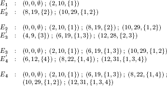
The last triplet (12, 31, {1, 3, 4}) of the set E₄ provides the results of solving (P):

COMMENT 8.8.– It is possible to deduce a solution and the value from the set E₄ of every problem in the form:

with y ∈ {0, 1,…, 12} (see comment 8.7). For example, for y = 9, the triplet (8,22, {1, 4}) provides the answer: v(P₄(9)) = 22 and .

8.6. Solution search by hybridization of branch-and-bound and dynamic programming

Almost all the first solution methods for the 0–1 knapsack problem were dedicated to tree searches using branch-and-bound. They differ in the search tree exploration strategy, the choice of the variable to branch, and the evaluation of the nodes, but also in the preprocessing of the problem (algorithms bounding the value of (P) and fixing variables). The common characteristic of all these methods is their lesser effectiveness, or even the explosion in their resolution time, when solving correlated instances (that is the couples (c_j, a_j) are neighbors [FAY 75, FAY 79]).

Based on the example given in [HOR 74], then in [AHR 75], for the subset-sum knapsack problem, whose objective is identical to the left-hand side of the constraint (for every j, c_j = a_j), which is more difficult to solve in practice since the pruning of branch-and-bound is ineffective, [PLA 85] proposed an algorithm for the problem (P) that hybridizes dynamic programming and branch-and-boundbased on the FPK79 method in [FAY 79, FAY 82].

This branch-and-bound algorithm FPK79 for the 0–1 knapsack (itself inspired by an algorithm designed for general integer linear programs [SAU 70]) constructs the search tree with the depth-first search strategy. The variable to branch is chosen according to the (static) decreasing order of the absolute values of the reduced costs at the optimum of (LP). Evaluation at each node N combined with fixing the variables x_j j ∈ N₀ (or N₁ respectively) to 0 (or 1 respectively) is performed by solving the Lagrangian relaxation associated with the optimal multiplier c_i/a_i of the Lagrangian dual of (P), where xi is the basic variable of (LP):

This choice is guided by the extreme simplicity of calculating its value:

since it can be done incrementally.

In this tree search, where, from construction, each variable x_j is fixed to the value as a priority (that is the one at the optimum of (LP)), these are the lower reduced cost variables, which are the subject of most of the research work, while the evaluation of the associated nodes is of very poor quality. This characteristic implies that the pruning tests for these nodes are inefficient and therefore a practically exhaustive exploration of the largest levels of the tree is involved. This leads to the idea of using dynamic programming for variables with small reduced costs in absolute value (instead of a tree search) since its complexity is independent of whether or not the data are correlated.

8.6.1. Principle of hybridization

The hybridization of branch-and-bound and dynamic programming therefore consists of partitioning into two the set of variables of the knapsack problem:

– the variables x_j, j ∈ D, whose reduced costs at the optimum of (LP) are the smallest in absolute value (the basic variable x_i whose reduced cost is zero belongs to these), the associated “core problem” being solved by dynamic programming;

– the other variables x_j, j ∈ I = {1,…, n} \ D, which therefore correspond to the greatest absolute value reduced costs, the solutions of the associated problem being explored using a branch-and-boundalgorithm and optimally completed by those generated by dynamic programming.

COMMENT 8.9.– This procedure of partitioning the data into two categories, already present in embryonic form in FPK79, uses the core problem concept introduced by [AHR 75] for the subset-sum problem, then used by [BAL 80], then used several times by [MAR 90], and, even more recently, for the multidimensional 0–1 knapsack problem by [BAL 08].

More specifically, the following core problem:

is first solved by the algorithm from section 8.5.2, which provides a list E_card(D) of feasible combinations of objects in the form T_J = (a_J, c_J) with J ∈ D and a_J b.

For each leaf f of the tree generated by branch-and-bound, this preliminary work is systematically made use of as follows: by denoting by N₀ (or N₁ respectively) the variables fixed to 0 (or 1 respectively) in this leaf f, it is sufficient to solve the problem:

Its optimal feasible solution is obtained (with a complexity O(card(E_card(D)))) by detecting the couple T_J* = (a_J*, c_J*) of E_card(D) such that:

which corresponds to the best feasible combination of objects of D that it is possible to associate with the combination of objects of I represented by the leaf f, that is .

In this way, by reducing the tree search to the objects with large reduced costs, we can expect to prune a large part of the 2^card(I) leaves of the search tree; for each leaf considered, the associated solution fragment (dedicated to the objects of I) can be optimally extended to a global solution (that integrates the objects of D) with a linear complexity that depends on the size of the set E_card(D), that has itself been established once and for all in O(card(D)b).

8.6.2. Illustration of hybridization

We go back to the instance:

whose ratios c_j/a_j are already sorted in decreasing order.

We find successively:

– relaxation of (P): U = {1,2}, i = 3, L = {4} and v(LP) = 35.75 with x^LP = (1, 1,3/4, 0)^t;

– greedy algorithm: x = (1, 1,0, 0)^t and v(P) = 29;

– variable fixing: the reduced costs at the optimum of (LP) are the following:

No variable of (P) can be fixed since:

COMMENT 8.10.– The Lagrangian relaxation of (P) associated with c₃/a₃ is the following problem:

which is:

whose value is naturally equal to v(LP) = 35.75 (see section 8.4).

– Exploring the solutions: taking into account the size of the instance, we assume that we can solve a problem with two variables using dynamic programming. We therefore envisage the following bipartition of {1, 2, 3, 4}:

   - D = {2, 3} associated with the two smallest reduced costs;

   - I = {1, 4} associated with the other reduced costs sorted in decreasing order of their absolute values.

We therefore first construct the set E:

of feasible combinations of objects (trivial here) relative to the core problem (section 8.5.2):

COMMENT 8.11.– It should be noted that the three feasible combinations of this list do not appear (since they are dominated) in the complete solution of (P) using dynamic programming (see set E₄ from the illustration in section 8.5.2).

Tree search is solely dedicated to the data of I and in each leaf k of the tree (the variables 1 and 4 are fixed to 0 or to 1, that is x₁ = ε₁ and x₄ = ε₄ with ε₁, ε₄ ∈ {0, 1}) a problem to be solved remains:

which is solved (with a complexity O(card(E))) by detecting the triplet (a_J*, c_J*, J∗) of E such that:

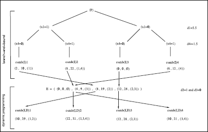
This leads to the scheme in Figure 8.10 which, for all the leaves of the tree, details (the branch-and-bound algorithm only develops part of them, see below) how tree search and dynamic programming are hybridized: each leaf corresponds (here) to a feasible combination of objects of I (comb(I)_j, j = 1, 2, 3, 4) that we only need to associate with the best possible combination of the set E to establish the best feasible combination taking into account all the objects, that is merging those of I and of D (comb(I, D)_j, j = 1, 2, 3, 4). The optimal solution is given by the combination comb(I, D)₂ of leaf 2. In this way we find that v(P) = 31 and x^P = (1, 0, 1, 1)^t.

Throughout the branch-and-bound method, the evaluation of each node of the tree is made by the Lagrangian relaxation associated with the optimal multiplier c₃/a₃ of the Lagrangian dual of (P). Thus the upper bounds of (P : x₁ = 1) and of (P : x₁ = 1 ; x₄ = 0) are equal to v(LP) = 35.75 (see section 8.4); that of (P : x₁ = 0) is obtained by solving:

whose value is 117/4 + d₂ = v(LP) − d₁ = 30.25.

Lastly, that of (P : x₁ = 1 ; x₄ = 1) is obtained by solving:

whose value is 117/4 + d₁ + d₂ + d₄ = v(LP) − |d₄| = 34.25.

The tree is explored depth-first in the (static) decreasing order of |d_j| by assigning each variable x_j to the value as a priority.

The solution of (P) is carried out in three steps.

Step 1: x₁ = 1 and x₄ = 0 (leaf 1) whose upper bound 35.75 is greater than v(P) = 29. The solution provided by comb(I, D)₁ = (10,29, {1, 2}) corresponds to that of the greedy algorithm and therefore to v(P).

Step 2: x₁ = 1 and x₄ = 1 (leaf 2) whose upper bound 34.25 is greater than v(P) = 29. The associated solution x = (1,0, 1, 1)^t provided by comb(I, D)₂ = (12, 31, {1, 3, 4}) corresponds to an improvement in v(P) which becomes 31.

Step 3: x₁ = 0 whose upper bound 30.25 is less than v(P) = 31. The algorithm stops without needing to explore leaves 3 and 4 of the tree. In this way we find that v(P) = v(P) = 31 and that x^P = x = (1, 0, 1, 1)^t.

8.7. Conclusion

The algorithm presented in this chapter is the end result of a series of works that started with a long collaboration between Fayard and Plateau [FAY 75, FAY 79, FAY 82], which was extended by further collaboration between Plateau and Elkihel [PLA 85], and more recently with Bourgeois [BOU 92] (program available at the address http://www-lipn.univ-paris13.fr/∼plateau/BPK). All or part of this algorithm has served as the basis for many results, also carried out in collaboration, that relate to extensions of the 0–1 knapsack problem with one constraint to non-linear cases or to cases with several constraints. More exactly, this concerns exact and approximate solutions of the collapsing knapsack [FAY 94]; exact and approximate solutions of the fractional knapsack with the conception of dualities and Lagrangian heuristics [NAG 00a, NAG 00b]; solving the surrogate dual of the knapsack with two constraints [FRE 93, FRE 96]; approximate solutions and reductions of the knapsack with several constraints [FRE 86, FRE 94, PLA 89]; and reoptimization in solving the Lagrangian dual of the knapsack with two constraints [THI 03, THI 05, THI 06]. In all these

Figure 8.10. Hybrid exploration of the instance with four variables

extensions, we must envisage instances with real number data; this version is also available at the address http://www-lipn.univ-paris13.fr/∼plateau/BPKr. Finally, for wider overviews, the reader can refer to [MAR 90] and [KEL 04] on the knapsack, and to the article by Fréville [FRE 04] on the knapsack with several constraints.

8.8. Bibliography

[AHR 75] AHRENS J., FINKE F., “Merging and sorting applied to the zero-one knapsack problem”, Operations Research, vol. 23, num. 6, p. 1099–1109, 1975.

[BAL 80] BALAS E., ZEMEL E., “An algorithm for large zero-one knapsack problems”, Operations Research, vol. 28, num. 5, p. 1130–1153, 1980.

[BAL 08] BALEV S., YANEV N., FRÉVILLE A., ANDONOV R., “A dynamic programming based reduction procedure for the multidimensional 0-1 knapsack problem”, European Journal of Operational Research, vol. 186, num. 1, p. 63–76, 2008.

[BEL 57] BELLMAN R., Dynamic Programming, Princeton University Press, Princeton, 1957.

[BOU 92] BOURGEOIS P., PLATEAU G., “Selected Algorithmic Tools for the Resolution of the 0-1 Knapsack Problem”, EURO XII – TIMS XXXI Joint International Conference, Helsinki, 1992.

[FAY 75] FAYARD D., PLATEAU G., “Resolution of the 0-1 knapsack problem: comparison of methods”, Mathematical Programming, vol. 8, p. 272–301, 1975.

[FAY 79] FAYARD D., PLATEAU G., Contribution à la résolution des programmes mathéma-tiques en nombres entiers, Thesis, Lille University of Science and Technology, 1979.

[FAY 82] FAYARD D., PLATEAU G., “An algorithm for the solution of the 0-1 knapsack problem”, Computing, vol. 28, p. 269–287, 1982.

[FAY 94] FAYARD D., PLATEAU G., “An exact algorithm for the 0-1 collapsing knapsack problem”, Discrete Applied Mathematics, vol. 49, p. 175–187, 1994.

[FRE 86] FREVILLE A., PLATEAU G., “Heuristics and reduction methods for multiple constraints 0-1 linear programming problems”, European Journal of Operational Research, vol. 24, p. 206–215, 1986.

[FRE 93] FREVILLE A., PLATEAU G., “An exact search for the solution of the surrogate dual of the 0-1 bidimensional knapsack problem”, European Journal of Operational Research, vol. 68, p. 413–421, 1993.

[FRE 94] FREVILLE A., PLATEAU G., “An efficient preprocessing procedure for the multidimensional 0-1 knapsack problem”, Discrete Applied Mathematics, vol. 49, p. 189–212, 1994.

[FRE 96] FREVILLE A., PLATEAU G., “The 0-1 bidimensional knapsack problem: toward an efficient high-level primitive tool”, Journal of Heuristics, vol. 2, p. 147–167, 1996.

[FRE 04] FREVILLE A., “The multidimensional 0-1 knapsack problem: an overview”, European Journal of Operational Research, vol. 155, num. 1, p. 1–21, 2004.

[HOR 74] HOROWITZ E., SAHNI S., “Computing partitions with applications to the knapsack problem”, European Journal of Operational Research, vol. 21, p. 277–292, 1974.

[KEL 04] KELLERER H., PFERSCHY U., PISINGER D., Knapsack Problems, Springer-Verlag, Berlin, 2004.

[LAU 79] LAURIÈRE J. L., Eléments de Programmation Dynamique, Collection Programmation, Gauthier-Villars, Paris, 1979.

[LAW 79] LAWLER E., “Fast approximation algorithms for knapsack problems”, Mathematics of Operations Research, vol. 4, p. 339–356, 1979.

[MAR 90] MARTELLO S., TOTH P., Knapsack Problems, Wiley, New York, 1990.

[MIT 64] MITTEN L. G., “Composition principles for synthesis of optimal multistage processes”, Operations Research, vol. 12, p. 610–619, 1964.

[NAG 00a] NAGIH A., PLATEAU G., “Dualité lagrangienne en programmation fractionnaire concave-convexe en variables 0-1”, CRAS : Comptes Rendus de l’Académie des Sciences de Paris, vol. 331, num. I, p. 491–496, 2000.

[NAG 00b] NAGIH A., PLATEAU G., “A Lagrangian decomposition for 0-1 hyperbolic programming problems”, International Journal of Mathematical Algorithms, vol. 14, p. 299– 314, 2000.

[NAG 00c] NAGIH A., PLATEAU G., “A partition algorithm for 0-1 unconstrained hyperbolic programs”, Investigación Operativa, vol. 9, num. 1–3, p. 167–178, 2000.

[PLA 85] PLATEAU G., ELKIHEL M., “A hybrid method for the 0-1 knapsack problem”, Methods of Operations Research, vol. 49, p. 277–293, 1985.

[PLA 89] PLATEAU G., ROUCAIROL C., “A supercomputer algorithm for the 0-1 multiknapsack problem”, in Impacts of Recent Computer Advances on Operations Research, R. SHARDA, B. L. GOLDEN, E. WASIL, O. BALCI, W. STEWART Eds, Elsevier North-Holland, p. 144–157, 1989.

[SAU 70] SAUNDERS R., SCHINZINGER R., “A shrinking boundary algorithm for discrete models”, IEEE Transactions on Systems Science and Cybernetics, vol. SSC-6, p. 133–140, 1970.

[SED 78] SEDGEWICK R., “Implementing Quicksort Programs”, Communications of the Association for Computing Machinery, vol. 21, num. 10, p. 847–857, 1978.

[THI 03] THIONGANE B., NAGIH A., PLATEAU G., “Analyse de sensibilité pour les problèmes linéaires en variables 0-1”, RAIRO/Operations Research, vol. 37, num. 4, p. 291–309, 2003.

[THI 05] THIONGANE B., NAGIH A., PLATEAU G., “Adapted step size in a 0-1 biknapsack lagrangian dual solving algoritm”, Annals of Operations Research, vol. 139, num. 1, p. 353– 373, 2005.

[THI 06] THIONGANE B., NAGIH A., PLATEAU G., “Lagrangian heuristics combined with reoptimization for the 0-1 biknapsack problem”, Discrete Applied Mathematics, vol. 154, num. 15, p. 2200–2211, 2006.

---

1 Chapter written by Gérard PLATEAU and Anass NAGIH (dedicated to the memory of Philippe BOURGEOIS).