7
Space–time Analyses and Modeling
In epidemiology, the availability of time for each event is a significant asset in spatial analyses. Taking time into account provides the possibility of ignoring proximity spatial relationships that should not be taken into account and that might falsify spatial analyses.
Retrospective spatio-temporal analyses essentially concern the following:
- – global spatio-temporal analysis (correlation between time and distance, spatio-temporal autocorrelation);
- – analysis of the movement of synthesis elements (mobile mean points);
- – search for clusters and local spatio-temporal hot spots and their evolution in time;
- – study of emergence and diffusion (finding the cases that generate diffusion, which are called index cases, studying the geometric parameters of diffusion);
- – pathway reconstruction, for the reconstruction of epidemics propagation;
- – spatio-temporal modeling, particularly modeling of epidemics.
Time series analyses are commonly used in many fields (especially in meteorology, natural or agricultural resources, oceanography, economics, etc.). In epidemiology, the retrospective spatio-temporal analysis always starts with a global temporal study: global trend, search for seasonal variations, cycle, etc.
7.1. Time–distance relationships
This is the first question, the preliminary stage allowing the consideration of a contagion relationship between health events. It involves an analysis of the spatial autocorrelation of time. Many tests have been developed for this purpose (Knox, Mantel, space-time K-functions, etc.).
For example, after having fixed a duration and a distance, the Knox test uses all the pairs of events to establish a table of contingency between the difference in time and the difference in space, then applies a χ2 test to see whether the values found are significantly different from a random distribution [KNO 64] (Figure 7.1).

Figure 7.1. Graph indicating which are the values of differences in distance (on the x-axis) and in time (on the y-axis) for which the Knox test allows the rejection of H0

7.2. Mobile mean points
The idea is simple: rather than considering the set of events, a mean (or median) center is considered for the events belonging to a temporal window with fixed duration. The movement of this temporal window in time results in a series of mean centers, which allows the smoothing and synthesis of the global movement of the phenomenon (Figure 7.2).

Figure 7.2. Movement of mean centers in time during a wave of avian influenza in Thailand
7.3. Spatio-temporal autocorrelation and clusters
7.3.1. Global spatio-temporal autocorrelation
Similar to the spatial autocorrelation examined in Chapter 5, the temporal autocorrelation T is expressed by a simple index:

The sum is extended to all the pairs of values temporally distant from k.
Spatial autocorrelation indices do not take time into account, and therefore they measure spatial autocorrelation without considering the temporal dynamics of the relationships between values and distances. Measuring the spatio-temporal autocorrelation comes down to simultaneously measuring spatial autocorrelation and temporal autocorrelation.
Several indices have thus been proposed [HAR 10, CHE 11]. The simplest idea is to limit the autocorrelation calculation to pairs of values that simultaneously satisfy a spatial condition (d (Рi,Рj) < d0) and a temporal condition (|t1 −t2| < h), by defining a spatio-temporal weight, such as:

Index distribution is always obtained by simulation. In the discrete case, simulation involves the permutation of the values (Xi, ti) of points among their spatio-temporal positions.
7.3.2. Local spatio-temporal autocorrelation
The same principle is applicable to local indices of spatial association, which then become local indices of spatio-temporal association.
7.3.3. Spatio-temporal clusters
Two types of studies use the search for spatio-temporal clusters: on the one hand, retrospective studies, where all data are available, and on the other hand, surveillance systems, where data are collected as the study progresses, and warnings are triggered when an “abnormal” situation is detected [ROG 97].
The search for spatio-temporal clusters relies on the same principle as for mobile mean points: in the search for the cluster, only the events of a temporal window are considered. The temporal window moves in time, which makes it possible to detect the appearance or disappearance of clusters. Spatial scan methods are the most commonly used [KUL 97].
Warning systems for infectious diseases use these methods; warning and surveillance systems often involve a real-time search for the occurrence of a spatial cluster.
It is at the beginning of an epidemic, when there are few events, and they are grouped due to their proximity, that clusters are statistically the most significant and their detection has the strongest impact on epidemic reduction.
The SaTScanTM software program is specialized in the search for clusters by spatial scan.


7.3.4. Statistical modeling: GTWR
Spatio-temporal extensions of the spatially weighted regression method GWR have been developed to include time in the analysis of non-stationary processes. The spatially weighted regression methods presented in Chapter 6 rely on the hypothesis of constant relationships in time. In order to take time into account, several authors have proposed to build spatio-temporal weight matrices for SAR or GWR models [WU 14, YU 14] using spatio-temporal distances to measure the distances between observations. Other authors have proposed the division of time into mobile temporal windows in order to determine the coefficients of GWR models using only the data observed in these temporal windows [FOT 15].
7.4. Emergence, diffusion, pathway
As already highlighted, when searching for the risk factors of a disease based on retrospective data, it is important to separate factors that pertain to a spatial relationship with the environment (mobile or immobile) from factors resulting from spatial relationships between agents. This is particularly important when the spatial relationships between agents are significant in the phenomenon, which is the case of infectious diseases. The analysis of the relationship between disease occurrence and environment by taking into account the set of cases involves the consideration of the contagion process in the simulation of random situations under null hypothesis, which is often difficult.
A further solution involves ignoring the cases due to relationships between agents (contagion). The idea is therefore to separate what corresponds to disease emergence (and therefore a priori due to an environmental factor) from what corresponds to diffusion by contagion, and to limit the analysis of health–environment relationships only to events that correspond to the emergence. On the contrary, diffusion by contagion can itself be influenced by the environment (by all the density-related factors: transportation, schools, markets, etc.). To study it, it is important to ignore the cases due to contagion.
Data that lead to establishing a direct causal relationship between one case and the previous case are rarely available. When the time and location of cases are available, these relationships can be reconstructed using a spatio-temporal calculation. The objective is double:
- – separate emergence and diffusion by proximity;
- – reconstruct the pathway of the epidemic and deduce its space–time characteristics from the pathway.
Pathway reconstruction or the characterization of emergence must be considered as modeling (Figures 7.3 and 7.4). Complementary data can also be used in the calculation, such as genetic filiations of pathogens, in order to refine the model and not limit it to purely geometric and temporal rules.
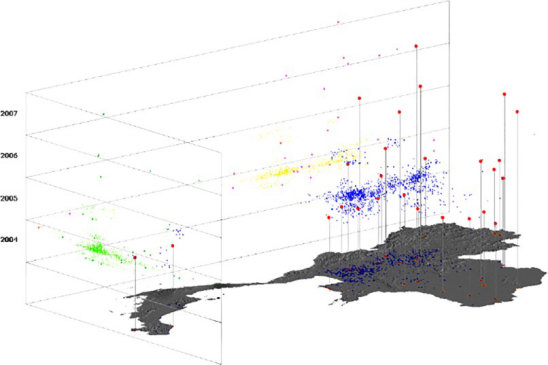
Figure 7.3. Avian influenza cases in Thailand, three-dimensional image. Time is represented on the z-axis. Red points correspond to the points of emergence (no previous cases for one month within a 50 km radius)
 |
Emergence and diffusion calculations are available with the menu: Calculate → Spatio-temporal calculations |

Figure 7.4. Pathway reconstruction for avian influenza epidemic in Thailand, from a point of emergence (index case). Reconstruction is made by the backward chaining depending on the distance between cases and an assumed propagation speed
7.5. Spatio-temporal modeling of health phenomena
7.5.1. Process modeling and simulation
Spatio-temporal modeling can be considered as the final stage in the analysis of a health phenomenon. Spatio-temporal modeling allows the approximation of the probability distributions of the phenomenon parameters, taking into account the model intrinsic characteristics and, by determining the spatial processes unfolding in the phenomenon, the simulation of its evolution in time. Probability distributions are obtained mathematically or by using simulations from the theoretical model and the initial conditions. In epidemiology, modeling has been used for several centuries (Figure 7.5).
A model is referred to as spatial if location (of agents or populations) is among the input variables, and as spatio-temporal if time is also an input variable. The model can only yield a global, non-localized result (such as global incidence, risk, transmission rate, etc.), a temporal result on phenomenon dynamics (for example, the global evolution in time of an epidemic), a localized result when location is an output parameter of the model (for example, an incidence in a geographical unit), or still spatio-temporal when the output dynamics is itself localized (for example, incidence evolution in a geographical unit in time).
From the modeler’s perspective, spatial analysis of the observed phenomena first aims to determine some characteristics and parameters of the searched model, and particularly the characteristics of the processes related to relationships and interactions among agents and between agents and their environment. Spatial analysis of the observed situations can also have a role in validating the model, comparing the spatial characteristics of the modeled situations with the spatial characteristics of the observed situation. Finally, spatial analysis of the results of a spatial model obtained from differential equations and diffusion equations may help in the characterization of underlying theoretical global spatial processes. All of the analysis methods presented in Chapters 5 and 6 can be applied to the result of a model.
The main theoretical models in the generation of events in spatial processes have already been mentioned: Poisson, Neyman–Scott, Matern, Cox, Gibbs, etc. Most of these purely spatial processes have been built for modeling continuous physical or environmental phenomena in a dense space (natural resources, meteorology, botany, etc.). In epidemiology, most of the observed phenomena are limited to a discrete support (places where the phenomenon is possible or those in which they are aggregated), and spatial analysis (of observed situations as modeled situations) provides indications on and characteristics of the underlying global theoretical processes, independently of the spatial distribution of the support.

Figure 7.5. The evolution of modeling methods in epidemiology (according to [MAN 16])
Spatio-temporal modeling differs from statistical modeling. The objective of statistical modeling is a mathematical formulation of a parameter or risk, depending on assumed risk factors, and the coefficients of which are determined by statistical or heuristic analysis that only relies on the observed data. Because it approaches the phenomenon as a whole, spatio-temporal modeling is a priori much richer. However, it should be realistic, and therefore it should take into account as many parameters as possible, considering a health phenomenon as a complex system, as described in Chapter 1. These parameters include spatial relationships and interactions between agents (hosts, vectors, reservoirs, pathogens) and between the agents and their environments.
When studying infectious diseases, spatio-temporal modeling is particularly useful in understanding and anticipating epidemics. Generally, it involves a characterization of individuals in various states (SEIR “compartmental” model: susceptible, exposed, infectious, recovered or deceased) and efforts are made to model major phenomena that support the passage of an individual from one state to another. When a model takes into account numerous processes, it can rapidly become very complex.
Modeling first of all implies knowledge and understanding of the operation of agents involved in the system. The large majority of models are assumed simplifications of reality. Mathematical solutions or simulations allow the determination of the distributions of probability of variables, the dynamics of a variable in time and sometimes the localization of the result in time and space, when the result of the model is itself spatialized [DIE 00, AUC 08].
Two large categories of methods are used in modeling:
- – A deterministic approach, which relies on differential equations (modeling the inputs and outputs of a state), and more generally an analytical approach of which the parameters result from the observed data and characteristics of the agents. Models that deal with populations instead of individuals have difficulty in taking into account complexity and particularly spatial relationships.
- – A non-deterministic approach, which directly models the evolution of agents, whose individual behavior is described by the rules that experts formulate based on systemic analysis (individual-based and multi-agent models). The state of each agent is calculated at each time step from their behavior, environment and relationships between the agent and the set of other agents. These models provide the possibility of a much more realistic description of the studied phenomenon, close to the complex system that finely describes reality. They make it possible to consider spatial relationships at each time step. These models involve heavy calculations and their use has been facilitated by the development of computational capacities. The main difficulties are rule determination and validation.
7.5.2. The deterministic approach of SEIR models
The SEIR model is specific to epidemiology. It characterizes agents by four different states: susceptible, exposed, infected and recovered. At each time step, susceptible subjects may enter the system, and recovered and deceased subjects may exit the system. A “compartment” is defined as the population of agents that are in the same state. The model relates to the dynamics in a population of the count of the agents, for each state; the result concerns only the evolution of the count of each compartment in time. Modeling involves the quantification of the number of passages from one state to another by unit of time, depending on the processes that describe the phenomenon.
All agents of the same type (host, vector, reservoir, etc.) that are in the same state are considered as identical and undergo the same processes in the passage from one state to another; a compartment is considered as homogeneous. Processes concern individuals, but the parameters describing these processes are evaluated by statistics on the phenomena observed on the populations, and therefore result from means or variances. Agent location is not involved in the modeling, which considers the population as a whole; individuals are subjected to the same environmental conditions, wherever they are, and interactions are expressed by processes that take into account the location of agents and of their interactions only by means or random processes. The model is expressed by a mathematical formulation, and the result is only determined by parameters and initial conditions. Random components can be introduced in the coefficients of some parameters by studying the variability in the observed data.
For example, the highly simplified SEIR modeling of malaria published by Ross in 1910 involves two types of agents: human individuals and (anopheles) mosquitoes, which can bite human individuals and transmit the malaria parasite or can become infected themselves if they bite an infectious human individual. Similar to mosquitoes, human individuals are grouped into two compartments: susceptible and infectious. Compartments are presumed uniform (all individuals have the same risk of being bitten by a mosquito and mosquitoes have the same risk of being infected). For each time step, the transfers from the compartment of susceptible individuals to the compartment of infectious individuals and vice versa are evaluated. An infected individual is assumed recovered after some time and joins the compartment of susceptible individuals. An infected mosquito is assumed to remain infected throughout its life, and all mosquitoes have the same life expectancy. This highly simplified model has nevertheless contributed to advancing two concepts that are essential for the strategies to fight against vector-borne diseases: the basic reproduction number R0, which corresponds to the mean number of individuals that an infected individual may infect, and which can be used to determine the evolution of an epidemic in a population; and the vector capacity, which summarizes all the characteristics of the vectors impacting the model and R0 [REI 13].
The initial Ross model has omitted many parameters (for example, latency times between infected and infectious state for both human individual and mosquito, duration of immunity, differences between symptomatic and asymptomatic subjects, etc.). In order to take these parameters into account, the model has been subjected to many developments [MKE 04]. Nevertheless, most compartmental models elaborated during the last 40 years are very similar to the Ross model, despite increasing awareness of the geographical, ecological and epidemiological complexities, which require the differentiation of socio-economic characteristics of the agents and the consideration of the environmental conditions that they are subjected to. Taking this complexity into account requires these models to be spatialized or individualized.
7.5.3. SEIR models and localization
The main critique that may be formulated of global SEIR models is specifically that they are global and they only consider means over a population, while the processes at play depend on individual variables. This once again highlights the ecological fallacy problem: for example, in the same population, the susceptible individuals are not necessarily those exposed, and approaching individual mechanisms by using mean values in a population may lead to errors; similarly, an R0 results from a global approach in a population and is a transmission mean per individual, but the reaction in terms of public health is very different, depending on whether the variance is low and the distribution is normal or there are several super-spreaders, or more generally a sub-population whose probability of disease transmission is far above that of the global population. This is indeed the case with many infectious diseases.
If the model is required to take into account the differences in the environmental, socio-economic or behavioral conditions that influence processes at the level of individuals, the individuals in the population should be differentiated depending on these conditions and more homogeneous sub-populations should be defined for these variables. Moreover, if the objective is to study the spatial distribution of the modeling result, the model should be “spatialized” and have as output a localization or a spatial value, and consequently sub-populations that are homogeneous in space, corresponding to aggregation into geographical units.
Fortunately, the variables related to the vulnerability of populations often have non-random spatial distributions. The same is true for many environmental risk factors. The solution is to define sub-populations of agents corresponding to a space division that reduces the intra-variance of the main hazard parameters and of vulnerability that is considered as immobile (population susceptibility and immunity, socio-economic conditions, environmental conditions), according to their importance in the model. As for mobile factors, they should be evaluated by a geographical unit of this division at each time step (for example, climate variables or contacts between agents).
Therefore, a division into geographical units should be found, which allows the definition of sub-populations that are expected to be more homogeneous with respect to environmental and socio-economic conditions, and which allows a different parameterization of the processes modeled in each sub-population by a classical SEIR compartmental approach. This is the usual problem of disaggregating a population into groups, with the minimization of inter- and intra-variances between groups.
To be realistic, spatialized SEIR modeling must also take into account the count transfers between the sub-populations in each compartment and therefore between various geographical units. Reaction–diffusion models are then used to take into account the propagation effect and the impact of population movements on disease persistence or extinction. The characteristics of these reaction–diffusion models are evaluated by spatio-temporal analysis of the observed situations. This brings us once again to the concept of metapopulation, of special use in ecology, with models for the management of species or for the modeling of prey–predator systems.
For example, most models of diffusion of an infectious disease must take into account proximity-based diffusion (adjacent units exchange agents in each compartment) as well as long-distance diffusion (representing long-distance jumps and new local occurrences). The rates of contacts between individuals, geographical connectivity between units and the spatial structures of the movements are essential parameters of diffusion models.
7.5.4. Non-deterministic approach of multi-agent models
Ultimately, it is possible to have complete disaggregation and the model could consider sub-populations with only one individual: these models are called individual-based models (IBM). When several types of agent are involved, these models are also known as multi-agent models (SMA). They have the advantage of considering the actual values of the individuals, avoiding any ecological fallacy and being able to directly address interactions and spatial relationships between agents. The main difficulty is, of course, in knowing the individual values of all agents’ parameters, which is generally impossible. In the vast majority of cases, the actual values are assessed by population survey, and then randomly assigned to agents depending on these probability distributions. Moreover, some elements related to individuals are difficult if not impossible to obtain, and are equally difficult to address in a survey, as mentioned in Chapter 1. This is the case of individual movements and also of some events with significant spatial variability.
Finally, these individual-based models can only be solved by a computer simulation; instead of equations built using a mathematical formulation of the process, individual-based modeling uses rules that apply to individuals, at each time step, to modify their attributes. The result of modeling is the statistical description of some variables, and mainly the count dynamics of each compartment in time. These models are non-deterministic to the extent that they cannot be solved analytically. Moreover, most rules involve random elements.
The spatialization of multi-agent models is rather simple, as it is sufficient to take into account the localization and have rules for the movements of individuals. On the contrary, it is very demanding in terms of the quantity of geographical data and especially of calculations. An evaluation of the environmental conditions to which each agent is subjected depending on its location (the corresponding rules being applied to it) is required at each time step. Spatial interactions between agents must also be evaluated (the corresponding rules being applied to them). Most systems use a simplified geographical reality in order to reduce time calculations (for example, solving these geometric calculations in raster form, the environment being spatially described as a grid).