Chapter 7
Using Wireshark and TCP dump to visualize traffic
Abstract
We focus on network traffic visualization using Wireshark and TCPdump. We give practical tips including using built-in analysis tools, as well as display and capture filters to filter traffic. We show how you can find and identify abnormal flows in the network.
Keywords
Wireshark
network analysis
display filters
capture filters
TCPdump
flow identification
One truth about security testing is that if you cannot see it, you may not be able to defend against it in the networks. This is where tools like Wireshark come in handy. What I will do in this chapter is show you tips and tricks for using Wireshark for the overall reason to give you another tool in the defense of your network. There are many resources on the net that will help you install and perform basic operations such as here (https://www.wireshark.org/docs/wsug_html_chunked/ChapterIntroduction.html). I will make one recommendation about install, and that is choose the 64-bit version of Wireshark if you have to choose based on your operating system. With the additional memory space available to 64-bit applications, Wireshark will be able to keep larger traces in memory. Visualization of traffic is a critical part of detection of exploits and, frankly, valid traffic in the network.
Understanding Valid Traffic in the Network
You cannot identify flows of attack in the network unless you understand what is valid in your network. To achieve this, we need to create a baseline of valid traffic. Now, when you create a baseline, you really do not know if the traffic you see is valid or exploited. The way to sort this out is to begin to understand what protocols, transports (TCP/UDP), and port numbers are valid and more importantly, what conversations are allowed and which ones are not allowed. For example, malware may use HTTPS to “Phone home” data it captured from a database. If you just captured traffic and only inspected the protocol you would use HTTPS on TCP/443. There is nothing suspicious there. When you inspect the conversation, you may see traffic attempts from an application server to the Internet. Since an application server should only talk to an SQL server and an HTTPS server pool, all within our network, this flow should be marked as suspicious.
As a general rule, when inspecting traffic, do the following:
Identify protocols in use over a long sample period (like a week).
Identify the flows associated with those protocols.
Match the addresses and protocols to what “should” exist in the network.
Log what is valid.
Retest often, use differential analysis to see what is different.
I will also point out that this information should be correlated with your IPS/IDS log information. Furthermore, you will need to do this analysis for each of your zones in your network. This will give you a solid foundation for understanding valid flows in your network.
Now we have to get practical and show how this may be accomplished for a zone. The first thing we have to do is pick the “Sniffing” point in the zone. In general, this should be as close to the core of the zone and/or near zone boundaries connecting the zone to other zones. You want to capture as many samples as you can when sniffing traffic. Once we have identified where we want to “Sniff” we need to bridge that traffic in a network “span” port. For this example, I will assume you are using a Cisco Catalyst switch, but your specific vendor will have specific instructions with the same effect.
Setting Up a Span Port
When setting up a span port, you need to be aware of some core things. First, the link speed of the span port should be greater than or equal to the maximum bandwidth of that which you are monitoring. For example, if your zone switch is forwarding 23 GBps and you use a 1 GB Ethernet link to span traffic to your Wireshark host, 22 GBps will be dropped. One way around this is if you are using VLANs, do an analysis study for each VLAN independently as opposed to spanning the whole VLAN trunk.
Example To set up a span port of a Cisco Catalyst 6k (IOS):
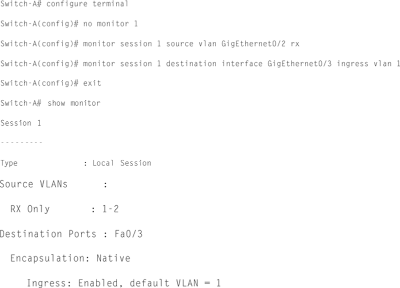
In this case, plug Wireshark into port GigE0/3 and you should be able to monitor traffic form port GigE0/2, bidirectional. Test this by starting a raw interface capture on Wireshark.
Using Capture and Display Filters
When examining traffic on the wire, unfiltered traffic is not very useful. Simply put, there is too much going on in the wire to make sense of it. Therefore, we must utilize filters to narrow the scope of what we are looking for across the network. To do this, we use display and capture filters on the traffic stream, with each filter rule set being different. A capture filter is an expression that determines if a packet will be forwarded to the capture file or discarded, based on a Boolean operand. To set a capture filter, in the main Wireshark screen, select Capture Options.
Then, click on Capture Filter. The capture filter has a name and a filter string (Fig. 7.1).
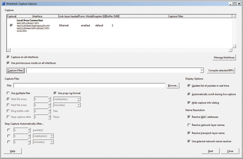
Figure 7.1 Wireshark Capture Filter Dialog.
Wireshark has some predefined fitters that are useful, but the real power is allowing you to build and save your own filters. Remember, a packet must pass the filter before it goes into the capture buffer (Fig. 7.2).
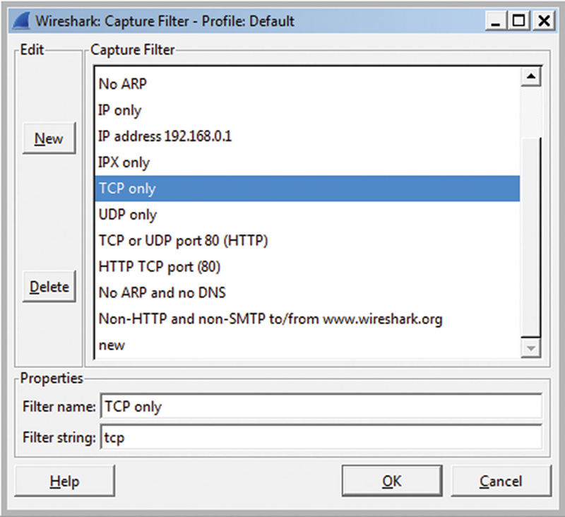
Figure 7.2 Wireshark Protocol Filters.
The best practice technique is to set Wireshark to capture traffic that is sourced or destined to subnets outside of the security zone (for example, you can use “not net 10.1.0.0/24” as a capture filter in Wireshark). For example, the datacenter backend will have SQL databases (such as Oracle or MySQL). Since we know that the only host that should talk to the database is the application server, and conversely, the database server should only talk to the application server, we can look for out bound traffic requests to detect flow path anomalies. Let us write a capture filter and examine what it does:
dst net not 192.168.0.0/24
This capture filter captures all destination traffic not bound for the 192.168.0.0 /24 subnet (assuming that is the local subnet). Given that the web server front in interface should be on a different zone than the backend network, if we see any out bound traffic events in the secure zone, that is a good indication of an infection.
We can also fine tune the capture filter to specific TCP port. Here is an example of a capture filter that looks for HTTP or HTTPS on the default ports.
tcp dest port 80 or tcp dest port 443
This example would be useful from the frame of reference of the user zone looking inward to internal server resources, such as a CRM system. Because we know that only HTTP and HTTPS protocols should be used, if we see other penetration attack attempts like a TCP port scan, we can write a capture filter for that as well.
(port not 80 or port not 443) and host 192.168.0.10
This compound capture filter is useful because if we examine it will place TCP or UDP packets that are not destination port 80 or 443 where the destination host is the web server front end. Now think about a TCP or UDP port scan. The penetration attack is going the scan though destination ports to see what listing ports are open. If it hits out trap by scanning a TCP destination port that is not 80 or 443 (and given that there are 65535 ports potentially available, this is likely). We can capture it and perform mitigation analysis. When building your filter statements, OR and AND become very powerful tools because you more directly narrow your filter to the most relevant information.
Here is a trick, since we are already using WinAutomation utility software, you can build an application that loops and looks for the Display packet count to increase, such as Fig. 7.3.

Figure 7.3 Wireshark Statistics Menu.
Basically, you create an infinite loop, capture the screen text, and compare it to the previous loop; if the new value is greater than the old value, then you can fire off an SMS or email to the administrator.
Example of Using Display Filters to Detect Reverse HTTP Meterpreter Shell
One of the advantages of having a tool like Wireshark that can dig through traffic is that you can alight it with filters that detect remote shells. In this example, we will leverage the fact that a Metasploit meterpreter shell uses an obsolete HTTP user agent string when attempting to open up a shell. Specifically, it uses “Mozilla/4.0 (compatible; MSIE 6.1; Windows NT).” First, there was no MSIW 6.1 and second a Host OS of ”Windows NT” without a version is suspicious.
Now, we can write a capture or display filter to detect this user agent string. The filter would look like

So if you see an HTTP or HTTPS request with this user agent string, it is a sure bet that it is a reverse shell. Now I have to point out some obvious facts, a reverse shell does not have to use this string. Therefore, sometimes it is better to look for matches that do not match the internal standard. For Example, the user agent string “Mozilla/4.0 (compatible; MSIE 6.2; Windows NT)” would not be legal because there is no “MSIE 6.2.”
Some Useful Display Filters
A TCP SYN flood attempts to open lots of TCP connections with no data, so we can create a display filter to search for TCP with no data. Specifically, the filter looks like

Then look for additional traffic on this TCP port/IP source and destination combination. If you see none, this is an SYN flood attack.
To look for TCP traffic with potential performance problems, use this filter:

This will help you identify slow TCP flows in the network. Another useful display filter for problem TCP connections is

This will show impairment events from the perspective of TCP flags and/or window size change. Retransmissions and slow TCP windowing can be a sign of intra-hop packet loss, or delay/loss at the endpoints, or too much aggregate end to end delay.
Using Custom HTTP Headers as a Backup Authentication
One trick to validate internal Web traffic is to add additional custom header to client requests. The additional header will be ignored by the server, but if you have a BOT or reverse shell, external entities will not know you ”Special” key. From this, you can create a rule that blocks any HTTP requests that do not have ”Your” header. You can also create a display filter to display http client source that does not have the header. To do this, if you are using chrome, it is to add in a plugin called “ExtensionNet Spanner.” This tool allows you to add in additional HTTP headers from the client, which you will use as a signature.
Here is a display filter to detect anomalous unsigned HTTP requests:

Assume that “aBh3828jsjs9” is your ”Signature.” So when the Display filter is applied and you see HTTP request that does not contain your signature, then you know you have suspicious traffic. Now, obviously this does not work for Internet facing client. But it should work for internal user hitting internal web servers.
Looking for a Malware Signature Using Raw Hex
Wireshark display filters also have the ability to parse through data in a packet and look for that pattern in the whole packet or in a layer within the packet. Here is an example display filter for inspecting TCP data traffic for a byte string in HEX:

This filter will look in the TCP data field for a specific string of bytes and whether the packet will be placed in the capture buffer. Since malware can sometimes be identified by a byte string, this can be useful for detection and mitigation.
Debugging SIP Register with Display Filters
You can also look for SIP specific traffic. In this example, we will look for SIP endpoint registration traffic. Here is the filter

This will allow you to see SIP registration packets in your network.
Using Built-In Wireshark Analysis Tools
Besides display and capture filters, Wireshark comes with a full set of built-in analysis tools to help you find and debug security and performance issues in your network. In this section, I will take you through the various tools offered in Wireshark and show you how to use them with an emphasis on security and performance debugging. In general, the most useful built-in analysis tools in Wireshark may be found in the “Statics” window. These tools will help you analyze packets that are in the capture ring (Fig. 7.4).
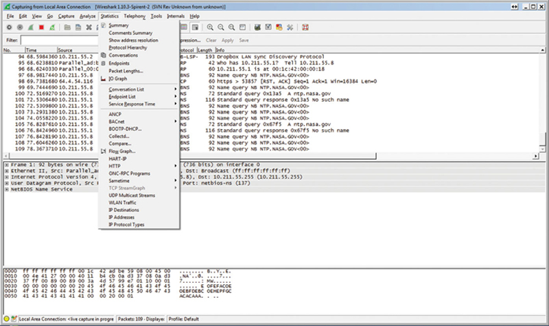
Figure 7.4 Wireshark Decode Window.
The first tool available is a simple protocols summary. This summary will give you capture file information such as file name and format, the file size and the encapsulation type, such as “Ethernet.” Next, the summary will give you the time of the first packet in the capture ring as well as the last packet and elapsed time. If you combine this with a composite capture filter, you can use this information to see when the first packet of interest arrives or network event occurred and when the last event occurred. This allows you you place context around an event. This summary will show for both captured and display filtered information about how many packets are in the buffer, time between first and last packets, average packet rate and frame size, size of the capture and alternative rate sin bytes/sec and Mbit/Sec. Also, this section will show you how many packets were ignored. With this information, you will know how well or poorly specific traffic is performing in the network (Fig. 7.5).
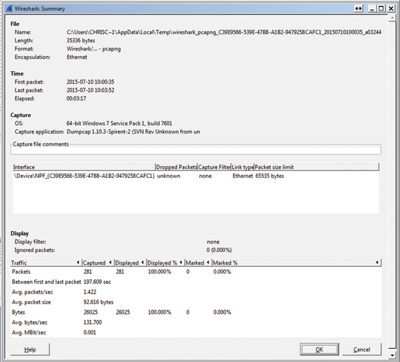
Figure 7.5 Wireshark Example Summary Page.
The “Show Address Resolution…” feature is a quick way of showing what Hosts were resolved by Wireshark, either by DNS or the local hosts file. This is useful in debugging to help you dereference a conical name or IP address in your analysis of the network (Fig. 7.6).
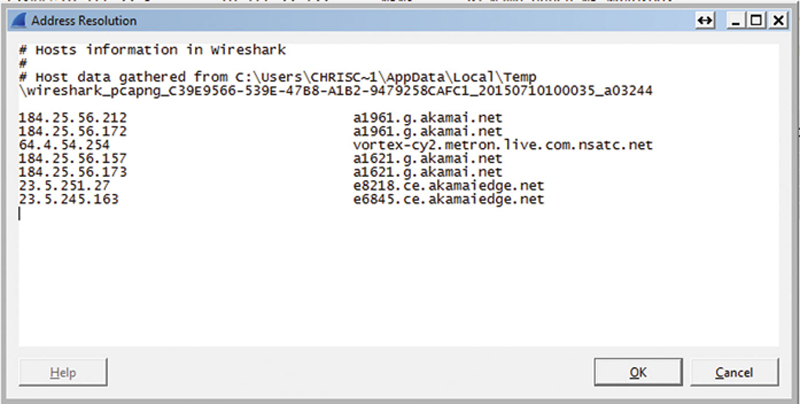
Figure 7.6 Local Hosts File.
The “Protocol Hierarchy…” feature is a really powerful tool. What it does is using the database of Wireshark dissectors (which are description files that show Wireshark how to detect and decode protocols), it applies an analysis of the traffic in the capture ring and shows you what protocols are active. The first thing the tool shows you is if there is activity on a protocol or not. Obviously, if you see a protocol that has any traffic and you do not expect it, that should raise a Red flag for you. Next, the tool will show the percentage of packets and bytes. Be very careful here, they will rarely add up to 100% if you just add the percentages. The percentages represent traffic encapsulations. Lastly, Wireshark will show you current bandwidth and peak bandwidth as a table of numbers (Fig. 7.7).
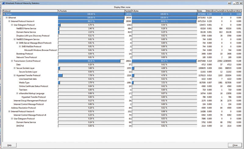
Figure 7.7 Protocol Distribution.
One of my favorite tools in Wireshark is the “Conversations…” tool. When launched, it will show you by OSI layer who is talking to whom. So I can look in the “IP layer” and see IP traffic pairs, but I can also look in Layer 4 TCP or UDP and see conversations. There are some check box options such as Name Resolution and limiting the conversations display to the display filter. If you are on a Layer 4 tab, the tool will show you the client address and source port number, the server address and protocol (like XRL or HTTPS). It will show the total packets and bytes, as well as by direction. Also, it will show you when the conversation began (relative time to Wireshark and the conversation duration). Finally, it will show you a bit rate by direction. Now, if I look at IP, UDP, and TCP, I want to look for suspicious traffic. This may include traffic where the source or destination is unexpected in that security zone, or a protocol that is being used that is not expected. Additionally, if there is a TCP or UDP conversation that has an excessive duration or total transfer bytes, that might be a malware bot “Phoning Home” data. In any event, it warrants a next stage of investigation (Fig. 7.8).
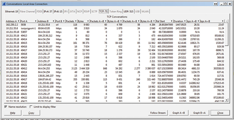
Figure 7.8 Protocol Summary Information.
Now, you can do some forensics with the conversation tool. When you find a conversation of interest, click on the “Follow Stream.” If you are on the TCP tab and you click a TCP conversation, the follow streams will show you the payload. By default, the tool will show you a HEX dump, with bidirectional traffic. To be convinced, I will switch the mode to ASCII. I want to filter the conversation by direction, I can do that using the pull-down, but I like to look at the 2-way conversation. Besides saving and printing the conversation, I use the find feature, which will search the conversation for key strings. Here is how you can use that. If you think a bot is phoning home data, and that this conversation may contain sensitive date, if you know of a keyword like “Credit Card” or your domain name (If the data you suspect being stolen is email addresses, search for the keyword). In addition, if you see source or more likely destination IP addresses that are unexpected, there is a good chance that you may have discovered a network trojan. You can use the following stream to further investigate the flow (Fig. 7.9).
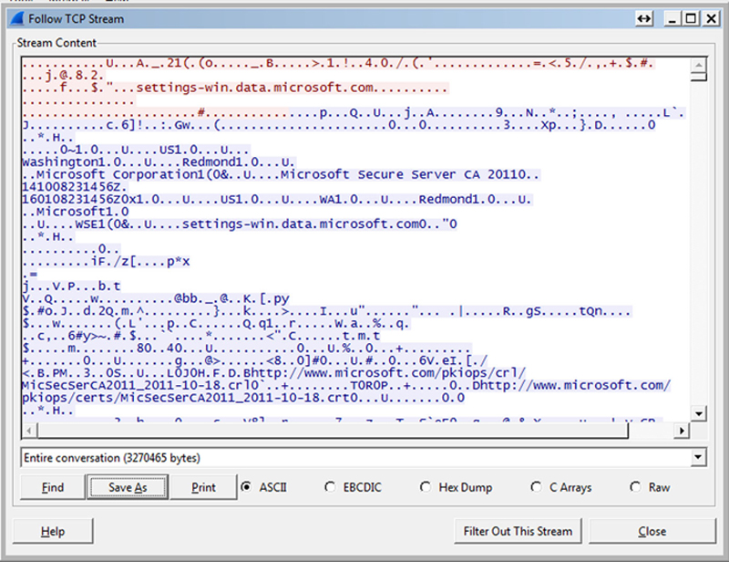
Figure 7.9 Following TCP Content.
In addition, you can click on Filter for this stream and Wireshark will build and apply a display filter for that conversation. Back in the main conversation dialog, you also have the option to graph TCP A- > B or B- > A, most likely meaning client to server or server to client. By right-clicking, you can see the packet associated with the information in the TCP flow. In the graph option > chart type you can choose from various views. Round-Trip time, Bandwidth, and Time/Sequence allow you to see various aspects of the TCP conversation. So, for example, if in Time/Sequence you see a shallow sloped line, then TCP may not perform at its potential peak across the network.
Using Endpoints Statics
As part of a forensics analysis of traffic it is very useful to see a list of endpoints from a security zone. Using Wireshark’s endpoint correlation tool is invaluable when performing tong term analysis of your network. There is one additional configuration you can make to endpoint tool to make it very useful, and that is applying a database of locations based on country, city, and ASN. To do this, quit Wireshark and go to MaxMind IP (http://dev.maxmind.com/geoip/legacy/geolite/). This database will help translate IP destination into Geolocations. Download and unpack the country, city, and ASN databases (IPv6 too if it is relevant for your network) (Fig. 7.10).
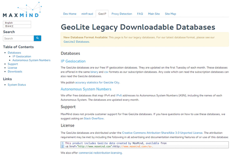
Figure 7.10 Downloading the GeoLite Database.
Now, under the Wireshark directory, create a folder called GeoIP, and place the .dat files there. Launch Wireshark and click on Edit > Preferences > Name Resolution. Here, click the edit button next to GeoIP Database directory. Click New, and browse to the …/Wireshark/GeoIP folder you created. Hit OK and Apply, then OK. Now quit Wireshark and relaunch (Fig. 7.11).
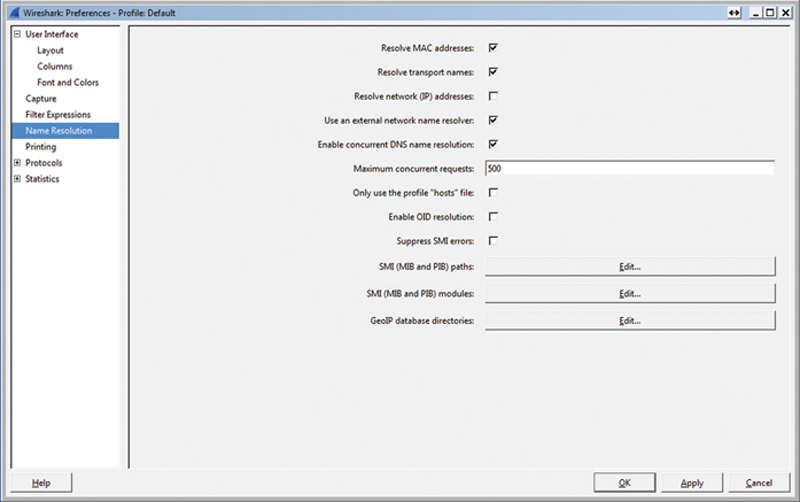
Figure 7.11 Setting the Geotag Preference.
The endpoint tool is very valuable when you have a large sample of packets over time. What you will see is a dialog box with tabs at the top, representing different protocol layers of traffic. If you click on the IP tab, you will see a Layer 3 view of conversations. Now, click on “Map” and you will see a geo location map of all of your endpoints (Fig. 7.12).
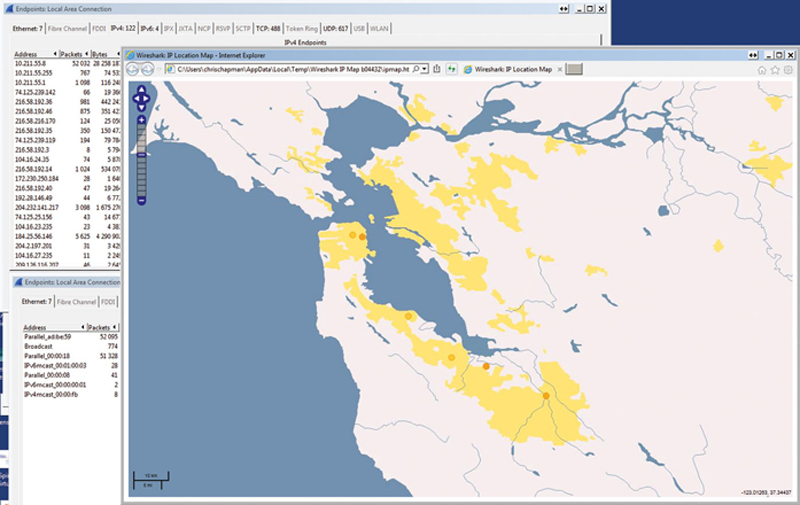
Figure 7.12 Example Mapped Dereferencing of an Address.
This feature is extremely useful in determining where potential hackers are attempting to route traffic (For example, a phone home of data attack might show an endpoint in eastern Europe. Since your organization has no endpoints in East Europe, it is safe to assume this is an attack). Maps also give you more visual representation of data to hand over to law enforcement if it is needed.
Now, say you see an endpoint of interest, if you right click, you can now have Wireshark automatically filter traffic based on this conversation. You can apply or prepare a filter. Preparing a filter will build the display filter string but not apply it, Apply prepares the string and executes it in the packet display. As an option, based on the endpoint tab you are on, you can choose selected. If this tab happens to be TCP, then it will write a display filter that includes both the IP and the TCP port number. For example, a TCP selected field would look like:

In this case, the display filter will display any conversation that has a source or destination IP in the siring AND has a TCP destination for 443. If you choose NOT SECLECTED, it negates this string to

In addition, you have option for “…And Selected”, “…Or Selected,” etc. When you choose this, it will append the current display String with an OR operator “||” or an AND operator “&&,” so you can build up complex display filters to narrow down the view. In addition, in the endpoints screen if you check “Limit to Display filter” and use Maps, you can visualize quickly conversations that may be attacks on the network. Finally, when you have a Display Filter you want to reuse, such as Fig. 7.13.

Figure 7.13 Example Display Filter.
You can hit “Save” and name it, it will show up on the toolbar for rapid reuse.
Determine Packet Length Distributions
If you use the “Packet Lengths…” static, you can see L2 packet size relative to a filter (or unfiltered). This is very useful when combined with a filter. If you filter on TCP only traffic and see packet sizes that are small, that may be an indication of an attack (Fig. 7.14).
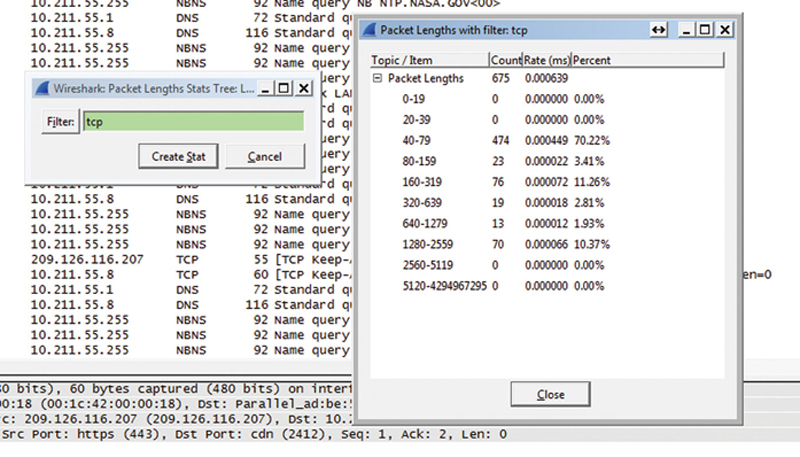
Figure 7.14 Example Summary.
In your display filter, you can then look for packets of a specific size using the display filter
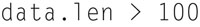
In this example, all packets greater than 100 bytes will be displayed. You can also create a capture filter that only captures small packets if you use the filters
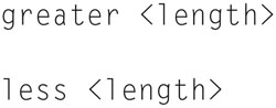
This is useful when tracking down packets of known size. For example, Layer 2 frame sizes of 576 are typical in a LAN.
Visualizing Performance With IOGraph
The IOGraph statics allow the user to graph up to five metrics at once to determine trend relationships. First, select “IO Graph” from the statics menu. Now, write a display filter to build a series. For example, you may want to graph TCP versus UDP bandwidth. So your filters would be “TCP” in Graph 1 series and “UDP” in Graph 2 series. Please note that you can apply any filter to a series, so you can get quite specific in what you are comparing. Now for each series, choose the graph type if you wish to smooth the graph (Fig. 7.15).
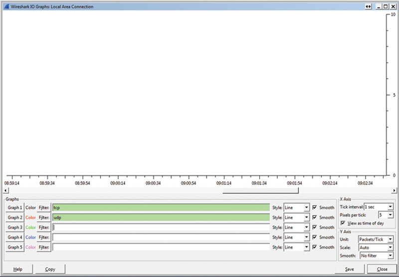
Figure 7.15 Wireshark IOgraph.
On the right hand side, choose the Tick interval (longer interval for longer analysis, shorter interval when complaining interpacket events and pixels per tick) on the X-axis. On the Y-axis, choose the units of measure and whether you wish to smooth the data and how the Y-axis values would be adjusted (auto) or fixed, or logarithmic.
Now you will see graphs drawing when traffic matched the filters. For example:
Also, when you click on the chart, the packet capture window will move to that timeframe, which is very useful. Another useful tip is the “Copy” button. When clicked, Wireshark will take the series data table behind the charts and copy it as a CSV to the clipboard. Here, you can paste the data and create more professional level of graphs. In addition, when you click on the “Graph {Number}” button, I can turn that graph on and off, when turning a graph on; Wireshark will recalculate values for that filter.
For advanced analysis, under the Y-axis > Unit, we can choose “Advanced.” What this will do is allow us to not only use a display filter to find packets, but then perform math operations on the set.
Here are the math operands:
SUM(*)—adds up and plots the value of a field for all instances in the tick interval
MIN(*)—plots the minimum value seen for that field in the tick interval
AVG(*)—plots the average value seen for that field in the tick interval
MAX(*)—plots the maximum value seen for that field in the tick interval
COUNT(*)—counts the number of occurrences of the field seen during a tick interval
LOAD(*)—used for response time graphs
So, for example, if I use this filter and expression and use the FBAR display type (Fig. 7.16):
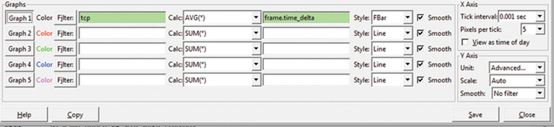
Figure 7.16 IOgraph Settings.
Then, I will chart the average frame delta time as a function of time. If I see the average time incrementing, it gives you information about a slowdown in the network. Lastly, you can click “Save” to save an image of the chart in a preferred image file format.
Using FlowGraph to Visualize Traffic
Sometimes, when you see traffic visually, patterns become obvious. With the FlowGraph tool, you can visualize TCP based or generic flows in the capture buffer. The first step in creating a flow graph is to create a display filter to narrow down the conversation of interest. The best way to do this is find a packet, such as a TCP segment packet, of the conversation and right-click. Click on Conversation Filter, than click on TCP. This will filter the capture ring to only this conversation. I also recommend that you right-click the first packet, and select “Set Time Reference.” This makes first packet times equal 0, and shows you more meaningful time offsets in the conversation. You will see a *REF* where you normally see the packet timestamp. This can also be toggled on and off (Fig. 7.17).
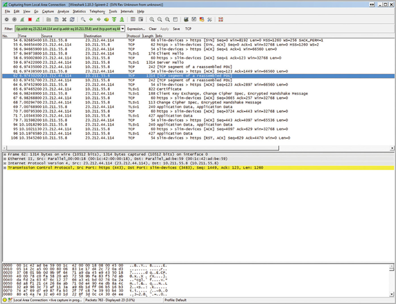
Figure 7.17 Packet Trace.
Now, click on Statics>Flow Graph and be sure to click on “Displayed Packets” and TCP flow. Now, sometimes you want generic flow, which is especially good at showing malware traffic, but in this case, we want to narrow our visualization down to a specific TCP conversation. When you click OK, you will see the TCP conversation (Fig. 7.18).
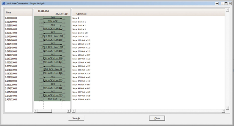
Figure 7.18 Example TCP Ladder Diagram.
Notice you will see the flowchart TCP flags and counters, such as SYN, ACK, and length. The Comments section will show the sequence number and Acknowledgment number, and you will see the timestamp to the left. If you hit “Save” a text representation of the flow will be save to a text file. If your display filter has more than single source and destination, you will see multiple vertical lines representing IPs and arrows showing flow of packets over time between those IPs.
Now, if you are cleaver with your display filters, you can show quite a bit of information in the flow graph. Say, you have a server and you want to see all traffic to and from the server, you could use the display filter:
If that host has a reverse shell and inside of the shell, the attack was scanning through the network; you would see this very plainly if you used “General Flows” option in the Flow graph.
Collecting HTTP Stats in Wireshark
Another very powerful feature of Wireshark is the ability to collect statics over a large sample period. A great example of this is the HTTP statics. Here the user can measure packet count, Requests, and Load distribution (Fig. 7.19).
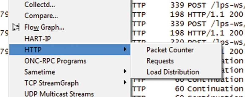
Figure 7.19 HTTP Analysis Options.
Packet count measures the HTTP request (like GET and POST) as well as the response types (4xx, 3xx, 2xx). This is useful for seeing if there is any unusual activity such as a “204 No Content” (Fig. 7.20).
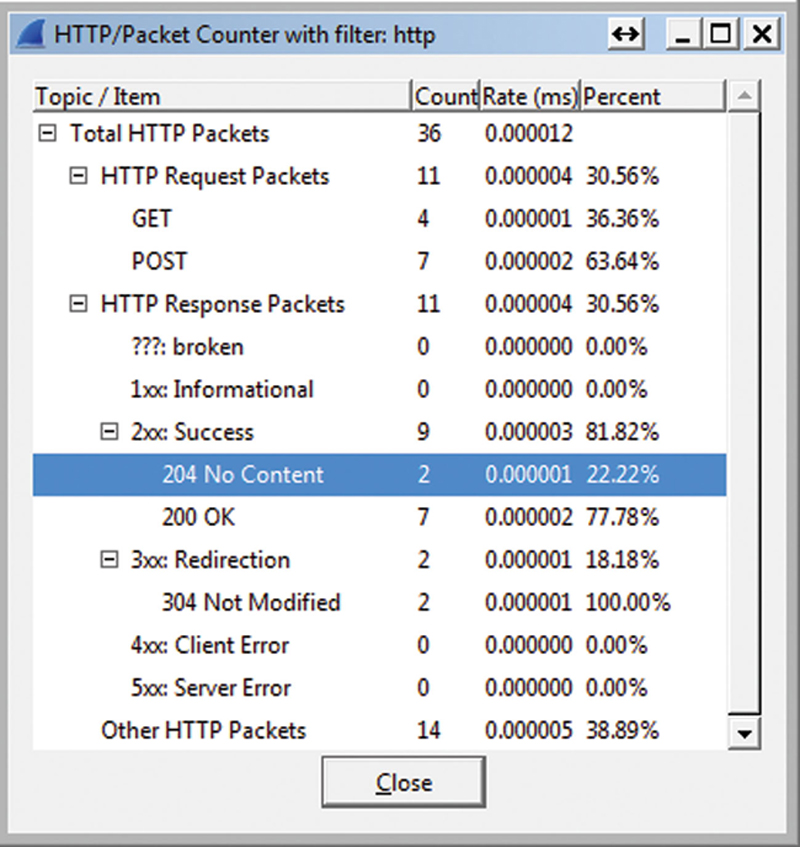
Figure 7.20 HTTP Summary by Response Code Example.
The HTTP requests will show you by server the requests that are made. Here is an example (Fig. 7.21).
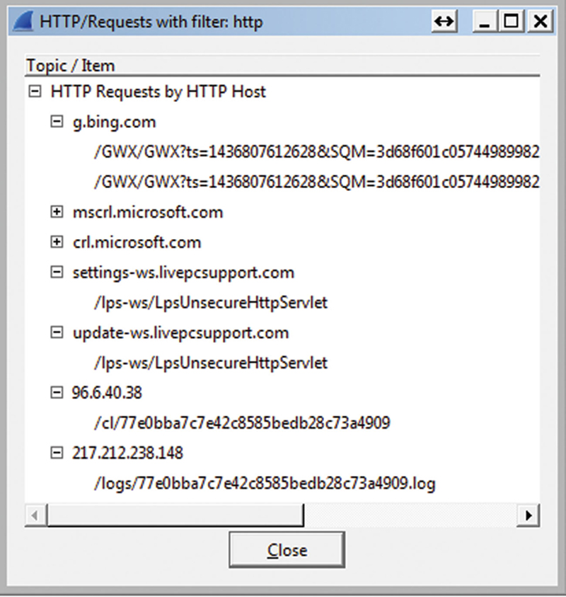
Figure 7.21 HTTP Example URI Analysis.
Finally, the HTTP Statics Load Distribution will show request and response as counts, bitrates, and percentage of traffic (Fig. 7.22).
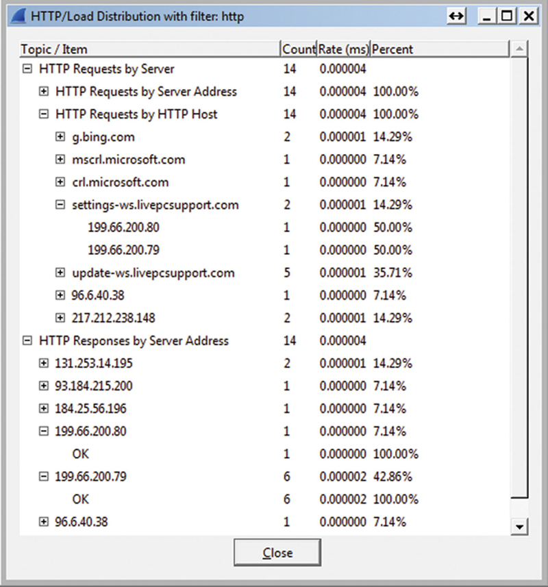
Figure 7.22 HTTP Load Distribution.
Using Wireshark Command Line Tools
You will get to a point when using Wireshark that you will realize that the GUI can only take you so far, and that the command line tools become in certain circumstances more useful to you. This is especially true if you are building automation scripts. Wireshark comes with a wire assortment of tool to help you understand your traffic from the command line. To use the command line utilities, go to windows Start, and type in CMD and hit return. This will open up a standard windows command prompt shell. Now, type in:
Now, type ’dir *.exe’ and press return, you will see the following programs:
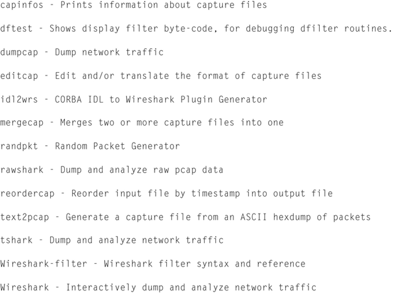
Now, look for ‘tshark.exe’ (Terminal Shark).
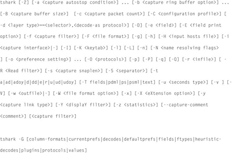
Tshark is a primary command line tool for Wireshark and is driven by the use of parameters. The full syntax for Tshark is:
The first step in using Tshark is to understand the Interface number of the desired capture interface. If you issue the following command:

you will see a list of available interfaces (explaining loopback). Here is an example of an interface list (Fig. 7.23):
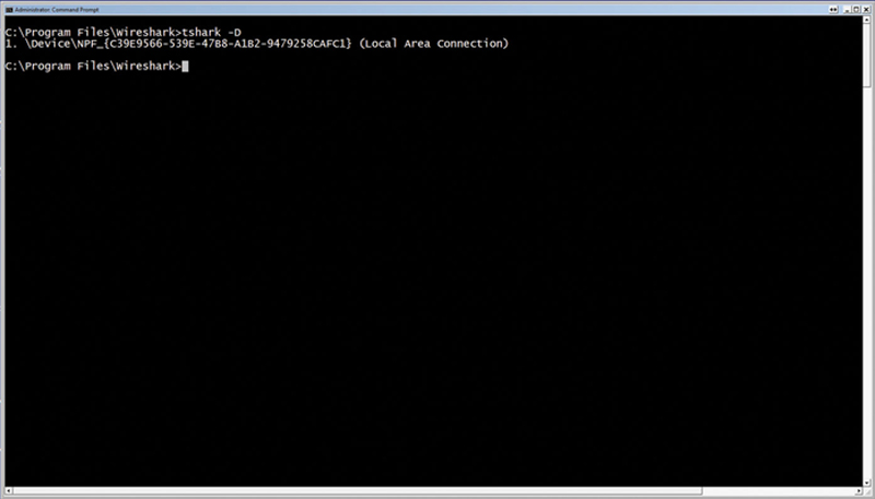
Figure 7.23 Using “tshark—D” to Show Available Interfaces for Capture.
Now, notice the number starting the line for “Local Area Connection,” in this case “1.” This is your interface number and it is very important.
So, to capture from Local Area Connection (Interface 1) and write the output to the file “out.pcap” with the field format of PCAP, use the following:

When this starts, you will see a packet count. You can press CTRL-C to stop capture and write-close the file (Fig. 7.24).
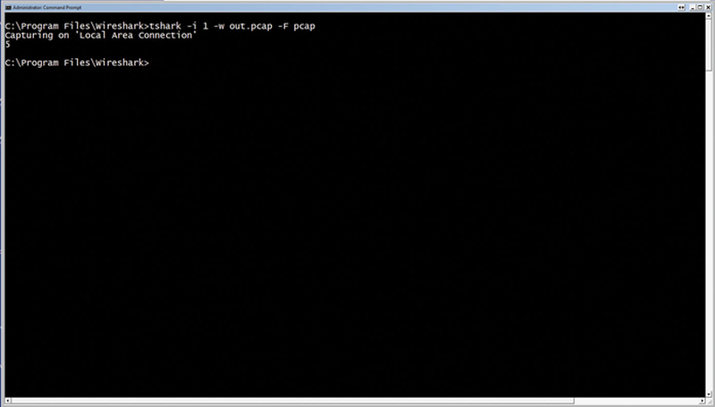
Figure 7.24 Start Capturing Using “tshark” for the CLI.
Now given that unfiltered capture is not very useful, let us demonstrate how to add a capture and display filter:

In this case, the capture filter, -f, will capture all Layer 4 traffic with source or destination port 80. If a packet comes into the port and does not match the criteria specified, the packet is discarded. Using the “-R” Display filter, only criteria that meets the filter will get “Displayed.”
The PCAP and PCAPng formats are binary, and it is sometimes useful to be able to extract frame data to a .CSV format for further processing. With Tshark, you can accomplish this easily. Here is an example of how to read in a .pcap file and extract information:

With this command, Tshark will “-r” read in the “sample.pcap,” you then tell Tshark in the output using the “-E” flag display option, Quite Fields, comma separated, write header names to top line of file. The “-T fields” flag tells Tshark which columns to include in the output. Each field is the field name (Trick: in the GUI, when you click on a field, in the lower left hand portion of the Wireshark window, Wireshark will tell you the field name) which is prefixed with the “-e” field. Finally, the output will be redirected from STDOUT to a file called “myresults.csv.”
How to Remotely Capture Traffic on a Linux Host
Sometimes, it useful to be able to remotely capture traffic on an interface that is not geographically near you. This may be accomplished using the command line tools for Linux. The first step is to run a password-less SSH environment on the local host.
Assuming you have OpenSSH installed from our previous chapters, issue the following command locally:
Now you need to copy the public keys to the remote host.
$ssh-copy-id -i ∼/.ssh/id_rsa.pub {Remote Host IP}
Just replace {Remote Host UP} with the IP of the remote host.
Next, you need to login to the remote host:
$ssh root@{Remote Host IP}
Now depending upon your distribution of Linux
Fedora/Ubuntu-based distributions:
$sudo apt-get install Wireshark
or from Debian distributions:
$sudo yum install Wireshark
Note: you will need to have Wireshark installed locally as well.
Now we are ready to start remote capture. This technique will remotely capture on all interfaces and the output is piped back into our local copy of Wireshark where we can then output to STDOUT, save as a PCAP, etc.
$ssh root@remote-host-ip ‘tshark -f “port !22” -i any -w -’ | Wireshark -k -i -
Merging/Slicing PCAP Files Using Mergecap
Many times when you capture traffic you will find that the direction of capture is one directional. Many times, you will only see the information of interest if you see information bidirectional. In addition, you may have a multisegment capture that you want to analyze as a set; this is a great example of where you would merge capture files together.
The basic format for merging is (Note the -v will output status in a “verbose” mode to STDOUT):
$ mergecap -v -w out.pcap pcap_source1.pcap pcap_source2.pcap.....
Now, you may ask how does mergecap know from which source file to pull the next packet and place in the output file. More specifically, what is the correlation variable. Mergecap will use the RX timestamp of the packet to determine order. This means that we have to manage a precaution before we can successfully timestamp packet, and that is manage time. It is really critical that all the source files be captured by devices that are synced to a common time source. For typical accuracy, you want to make sure your capture devices are synced with your internal NTP server (which is it’s self synced off of GPS). Do not point to more than one NTP server, either. Also, as a rule, do not use USB to Ethernet adapters for timing specific function. The internal latency of USB is not precise enough for our work. Once your capture devices are in-sync with a common time source, then we can start multisegment capture. When you merge traffic, then you can use tools like Flow Graph and display filters to analyze the traffic across a set or simply bidirectional traffic between a client and a server.
Getting Information About a PCAP File Using CAPINFOS
Capinfos is an application that gives you metadata about a capture file. The basic format of the command is
$capinfos {filename.pcap}
For example (Fig. 7.25):
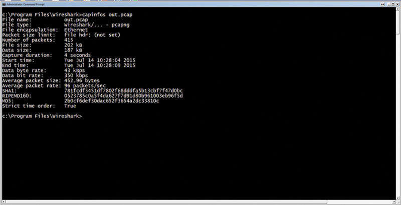
Figure 7.25 Example CAPINFO.
This will show start and stop times, files size, data size, encapsulation type, data rates, and checksums.
The useful nature of CAPINFOS is when you fine tune flags, like just showing data rate, in combination with a shell script and tools like GREP. Using data from CAPINFO, you can grab a returned value and variablize in your script. Here, you can loop across the variable and perform a comparison analysis to a known good value.
Editing a Capture File with Editcap
Editcap is a very powerful addition to Wireshark, because it allows the user to manipulate a capture file. For example, here are some things you can do with editcap:
• Find and include/exclude packets of interest based on content.
• Slice the parent capture into subcaptures.
• Translate formats.
• Edit content.
For example, if you want to edit out lines from a PCAP file you can use the following command:

This will output all packets, excusing the first 20 packets.
Also, if you want to include multiple ranges of packets in your output you can use the following command:

In this case, the output file will only contain packets 1–20 and 200–300.
A very useful feature of editcap is the ability to see what packets arrived during a specific timeframe. With this feature you can trace back detected problems from a firewall or IPS/IDS device and see the traffic at that moment. The format for this is shown in the following:

Also, another nice feature is the ability to add time compensation to packets in a file. You can add or remove time from packet. Here is an example of adding 30 minutes to packets in a file:

and in this example the user can remove 30 minutes of time per packet using the following format:

One of the main uses for this is to align the first packets timestamp when different capture sources cannot be properly time synced (say a one-directional remote capture in a foreign office). If you alight the packets by comparing timestamps and adding a compensation, you can merge the capture files for analysis.
Sometimes there are duplicate packets, especially after a merge. You can use editcap to remove duplicate packets using the following command:

Sometimes it is also useful to split a capture file into parts; you can do this by issuing the following example:
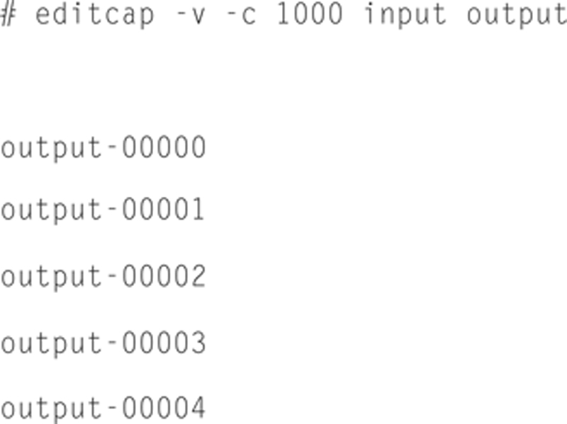
In this example, the input file will be broken up into 1000 packet files with an output name postfixes with the segment number until the source file is fully extracted.
Using TCPdump
TCPdump is a very powerful analysis tool. It is very similar to Wireshark in that it allows you to inspect traffic, but being a command line tool, you have many options for parsing the data. In addition, TCPdump lends its self very well when combining packet sniffing with automation of BASH scripting. First, we need to install TCPdump. TCPdump is already installed on Kali Linux, but if you happen to be using Ubuntu, you can issue:

You can test to see if it is installed by simply typing “TCPdump” and return. If you see packet information, TCPdump is installed. You can exit capture by pressing <CTRL > -C.
The first command you can execute is a simply summarized capture output to the screen using:
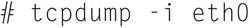
And you will get (Fig. 7.26):
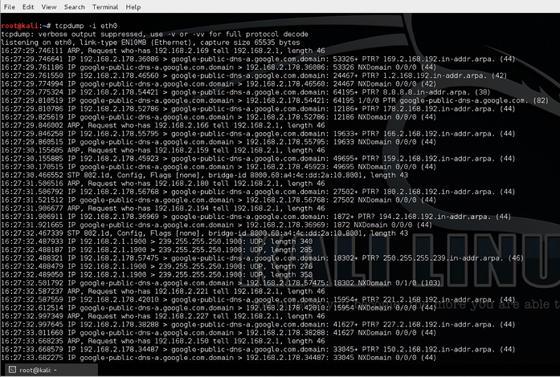
Figure 7.26 Example of TCPdump.
Here TCPdump will capture traffic from interface eht0 and display it to the screen. Note, if you use “-i any” then all interfaces will be used.
Now, we can capture more detailed information about traffic using
And we will get Fig. 7.27.
Figure 7.27 Example Packet Dump of Information In Normal Mode.
If we add the -ttt flag, we can then timestamp out traffic. With this you will get timestamps at the beginning of the packet, for example (Fig. 7.28):
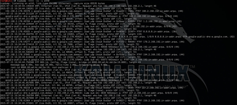
Figure 7.28 Example of Packet Dump in Verbs Mode.
If we use the -r flag we can output to PNG
# tcpdump -r out.pcap
To get the most decoding, use the following example:
and you will get Fig. 7.29.
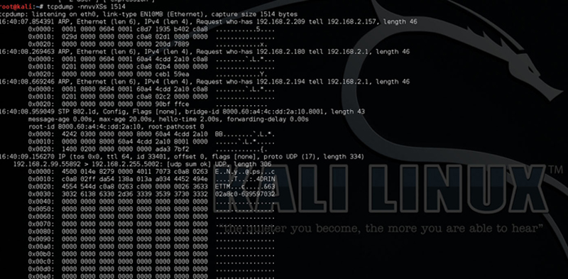
Figure 7.29 Hex and ASCII Decode of Packet.
Filter Captures with TCPdump
TCPdump like Wireshark is most powerful when you can build compound statements to filter capture to conversation of interest. If you want to capture from a source where the destination port is a set you can use:

In this example, the source must be 1.1.1.1 and the destination port must be either 80 or 443. You can also exclude protocols. For example:

This example shows a verbose capture from source net 1.1.0.0 where the destination traffic is not SSH.
To show all TCP URGENT pointer packets, use:

Or show all TCP SYN flags set to 1:

As you have seen, it is possible to AND, OR, and NOT filters together as well as order the expressing using parentheses. TCPdump, when combined with other Linux utilities like grep, becomes a powerful tool. TCPdump when combined with other Linux utilities like grep becomes a powerful tool.
For example:

This example will take the output of TCP dump, which is filtered to look for TCP port 80) and pipe the output to “grep,” with using the -e flag will look for “http“ and will write the output to tcpdump.out.
Summary
I covered how to use popular open source tools to help visualize traffic. With Wireshark, you are able to see traffic flows, traffic content, and how they are intermixed. In addition, analysis tools within Wireshark allow you to look at flow performance and characterize TCP based flows, which is useful for identifying slow or impaired TCP connections. TCPdump is a powerful tool for capturing, filtering, and analyzing TCP in detail. Both tools, together, allow you to debug real-time network issues.