Chapter 10
Traffic performance testing in the network
Abstract
We show how you may use open source tools to measure network performance. We cover key performance topics like streams and flows, as well as how to set them up and measure them. Last, we discuss how to interpret results.
Keywords
network performance streams
flows
traffic analysis
Whether you are evaluating a new device for the network, testing new code before deployment, or debugging network issues, having the ability to generate meaningful traffic and analyze it becomes critical to the smooth function of the network. I will show you how you can use open source tools to generate and analyze performance data across the network. First, you need to understand a few basics about performance testing. First, the general premise is that you choose a System Under Test (SUT) and declare that to be the outer edges of testing, with boundaries at Ethernet ports. Everything between the test ports is treated as a system. So, if your SUT spans multiple devices, then that chain becomes a system (potentially to test interoperability). Next, we have to discuss meaningfulness of traffic. The traffic patterns in your network are by definition the most meaningful to you. You will test an SUT in two ways. First, we place “Streams” across the SUT, assisted by QoS policies such as L3 DiffServ or VLAN tags with Class of Service (COS) set. The purpose of this kind of stateless traffic is to determine if pathways across the SUT can bare traffic. For example, if you see 10% packet loss at a high code point, say DiffServ AF41, then there is no point in further testing, because it would be a waste of time. Conversely, if the “Streams” are clean, then that gives you a green light to test with more stateful traffic. Remember, Stream testing will never tell you if your users will have a great experience, it can only tell you a course understanding if you might fail.
Another point I get asked a lot is why test at all? Is it not the vendor’s job, and did not they give me a datasheet with test results from RFC 2544? To answer this, is yes, all vendors test their equipment. The problem comes in that there is no guarantee that they tested well. Also, most certainly they did not test your specific patterns in their test plans (unless you are giving them millions of dollars of business each year). If weigh this against the absolute necessity for the production network to work, be reliable, be predictable, and be resilient, testing your specific patterns is a pretty inexpensive insurance policy.
Bandwidth, Packet Per Seconds and RFC 2544: Avoiding the False Positive
Every vendor will quote bandwidth, packets per second, and give you a datasheet with RFC-2544 results. The quote performance seems like a simple way to compare and contrast vendors. The main problem with this is that these numbers most likely will not represent the performance in your network because of how the test was performed, the difference in traffic patterns between a hypothetical network topology and your topology, and fixed frame and load sizes which are constant in measuring the SUT, but variable in your production network. RFC-2544 is fundamentally an engineering system test of the SUT. Once the elements of the SUT are integrated, RFC-2544 uses a Go/No go test. It is not intended to go on a datasheet, and can drastically lead to false sense of acceptance about the quality of the SUT. There are many reasons for this including over simplified traffic pattern, no QoS, and no real alignment to your network. What about packets per second. To be honest, this number is even less relevant than bandwidth. Generally, they test with very small frames (64 bytes) or an iMIX. I am not sure why “line rate” 64 bytes pps matters in a production network; you will never see that pattern in real life. The bottom line, thank the vendors for their datasheet, then “File it” away in the “Interesting, but need more information” folder.
Optimal Testing Methodology
If you do not understand the flows in your network (Allowed/Disallowed Services, their protocols, source and destinations nets, how this all changes over time), then you have no chance of characterizing your network. Spending time understanding how traffic flows from net to net, what flows, how they flow, when they flow, what policies they should follow is the best way to start. You need to characterize this traffic into two distinctive datastores. First, you need to characterize streams. This includes source and destinations nets, QoS levels used, Layer 4 protocols used and their destination port numbers, and how these floes ramp up and down through the day.
For example, a well-documented stream may look like:
From 10.1.1.0/24 to Server pool 10.2.1.0/24, TCP ports 80 and 443 are observed. This matches a DiffServ QoS policy and that traffic is marked as AF31 priority. This traffic is nominal (100 kbps) at night, but spikes to 500 Mbps between 8 am and 11 am, and on average is 300 Mbps from 11 am to 5 pm
This example fully documents a stream, and will allow us to build test traffic to model this across our desired SUT. Now, there will be multiple streams in play simultaneously, so build a “rule” for each observer stream. Streams will be overlaid forming our meaningful test pattern.
The second bucket you need to fill is actual captures of the streams. We will use this to play back across the SUT and measure if the device and its configuration are optimal. This traffic will fully stimulate up to layer 7 in the device (for example, a deep packet inspection firewall with logging turned on). By using your captures from your network, the traffic patterns now become alighted and meaningful, as opposed to generic.
Using the methodology of testing the pathways (Source/Destination nets + QoS marking + L4 Protocol header) quickly identifies and eliminates obvious course errors, and then testing with specific traffic gives us fine tune data about how the SUT will react in the production network. It should also be noted that this technique is not just for new devices, but also for new code or firmware for existing devices. As a best practice, no device or code should enter the network unless it has been meaningfully tested and verified because in the end, it is your business that is riding on top of the network. Here, failure is not an option.
Testing with Streams: Ostinato
Ostinato is a multistream open source traffic generator that is useful for testing streams and their respective pathways across an SUT. The tool allows the user to build up packets and schedule them out a test port. The analytics are a bit basic, only giving you port-based statics, but we will use other tools later in this chapter for analysis. The first step we need to do is install the tool. For this, I will choose to use Ubuntu Linux.
After you build Ubuntu, make sure all the based OS and packages are up to date. For this, open up a terminal window and type the following:
sudo apt-get update
sudo apt-get dist-upgrade
This process may take a while depending upon how out of date you are (You should always use an LTS version of Ubuntu, if you have the option).
Now, to install Ostinato, from the terminal, type
sudo apt-get install ostinato
Now to launch Ostinato, type the following:
sudo ostinato
When the tool launches you should see the following (Fig. 10.1):
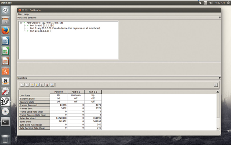
Figure 10.1 Main Traffic Generator Window.
Under the ports section, you will see a tree containing a list of psychical test ports (like eth1, eth2, etc), Loopback (lo) and “any” for multiport capture. These ports are grouped under a “Port Group.” If you want to cluster multiple traffic generators across the network into a virtual chassis, you can add additional port groups. To do this, you need to have Ostinato running on the remote generator. Then, click on File > New Port Group. Type in the IP address of the remote generator and the listening port number (default is 7878). This allows you to control multiple endpoints from a central GUI instance.
Now, right click on a generator port and select port config. You will see Fig. 10.2.
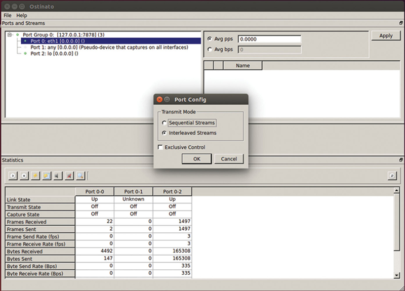
Figure 10.2 Choosing How Streams Are Generated.
Sequential Streams means that you set a port rate and the traffic generator will send one packet from each stream in a round-robin fashion. This mode is not useful for our needs. Interleaved streams means that you can set the rate per stream and the tool will determine from which stream to pull the next packet to assure the rates are as configured. Exclusive control means that only I have the privileges to this port. Click Interleaved Stream and OK.
To the right you will see the (Initially Blank) stream list. To add a stream, right click and “Add New Stream.” Click on the “Name” field and name the stream accordingly. A stream name should be descriptive including the Service, Transport, and DiffServ (or VLAN) information, for example Fig. 10.3.
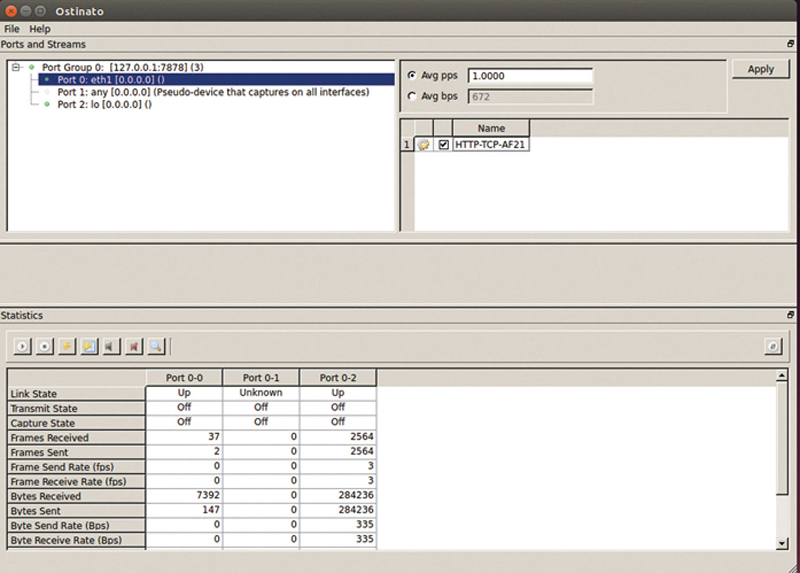
Figure 10.3 Example Results Window.
Good naming practices will keep larger configurations manageable. Now we need to configure the stream. Click on the “gear” icon next to the stream to open the editor.
You should see Fig. 10.4.
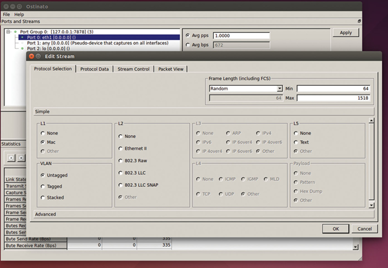
Figure 10.4 Packet Properties Window.
The protocol selection section allows you to select the layers of the packets that will be sent out of this stream. In the frame length section, you have the choice of fixed frame size, Increment, Decrement, and Random. For nonfixed frame sizes, you are asked to pick an upper and lower bounds for sizes. Standard valid range is 64 bytes to 1518 bytes for Ethernet, you can generate Jumbo frames (usually 9022 bytes), but you need to configure support in Linux for >1518 byte frame.
In Ubuntu, to configure Jumbo frames, at a terminal window before using the traffic generator, type:
sudo ip link set eth1 mtu 9022
sudo service networking restart
You can also type the following to verify the MTU:
ip link show eth1
“Simple” allows you to rapidly choose options for layers. For L1, choose “Mac.” If you are doing CoS and VLAN-based QoS, choose Tagged. If you are in addition, using Q-in-Q VLANs, choose Stacked. For L2, choose “Ethernet II.” For L3, you are most likely going to use “IPv4” unless you are implementing IPv6. In the L4 section, choose TCP or UDP according to the desired transport. Under the payload section, we can either type in or paste from a packet trace an upper layer protocol event (like an HTTP GET request). We can also choose our desired padding. “Advanced” allows the user to add more complex header classes such as IPv4 over IPv4. It is pretty unlikely you will need these headers (Fig. 10.5).
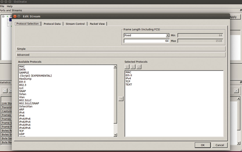
Figure 10.5 The Packet Structure Editor.
Next, click on the Protocol Data tab to edit the layers. You will notice that you can click through each layer by clicking on the layer button. You basically want to start at the top and work down. The first Layer is “Media Access Protocol.” In this layer, you will type in the L2 Source and Destination MAC address of the stream. You can put any value you want, but there are two caveats. First, the traffic generator cannot ARP for a router interface and fill in the destination address automatically, so if you plan on routing the packet, be sure the destination MAC address matched the router L2 MAC address. Second, be sure not to use an L2 multicast address (unless you are testing that specifically). The range to avoid is 01:00:0C:CC:CC:CC to 01:80:C2:00:00:0E. Under Mode, you can set the address (like the source MAC address) to Fixed, Increment, and Decrement. If you choose Increment or Decrement, you will be asked for a count and a step (eg, skip every eight addresses). Making the source L2 Address increment across a large number of MAC addresses (AND corresponding source IP and destination IP address) is a great way of filling the ARP table of the SUT and performing a better “Worst case Scenario” test (Fig. 10.6).
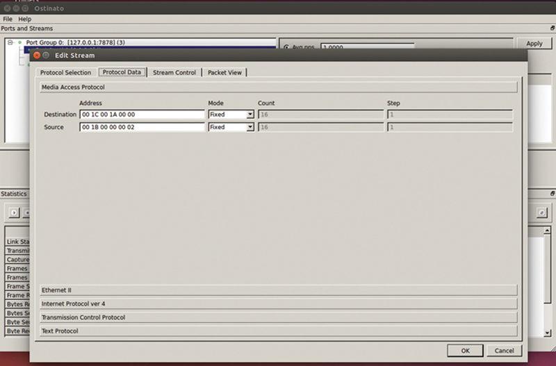
Figure 10.6 Address Editor Example.
Under “Ethernet II” check the Ethernet Type and verify “08 00” is inserted, this is the hex code for IPv4 as the next layer (Fig. 10.7).
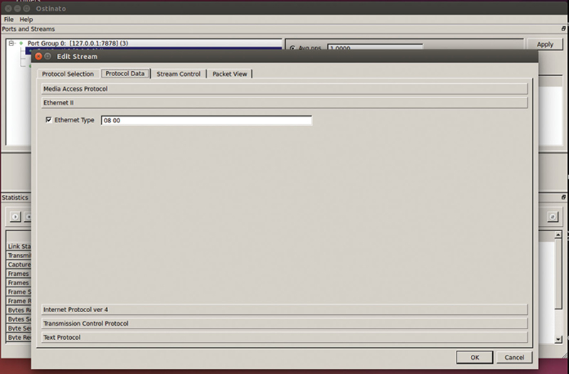
Figure 10.7 EtherType Selector Example.
Under “Internet protocol ver 4,” you can edit the IPv4 header. Some fields are automatically filled in such as Checksum and L4 protocol (“06” is the hex code for TCP). You have the option of setting fragments if you choose, or Don’t Fragment bit. Now type in the source and destination IPv4 Addresses. In addition, consider changing mode to Increment to cycle through a large set of addresses (by setting the count and mask). Note, the tool will automat skip over network and broadcast addresses based on the mask you specify. Next, you will need to set the L3 ToS byte. The field is just the raw HEX, so unless you want to build the hex bits by hand, I would recommend using a ToS/DSCP calculator (Note: No one really uses ToS anymore, so focus on DSCP). If you go to http://www.dqnetworks.ie/toolsinfo.d/dscp.shtml and scroll down to the DSCP section, you will see the binary or decimal equivalent to each DSCP level. Just use a scientific calculator (like Windows calculator in programmer’s mode) to convert the decimal or binary to hex. Place that value in the ToS field (Fig. 10.8).
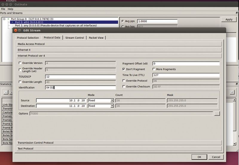
Figure 10.8 Stream IP Address Editor.
In the “Transmission Control Protocol” section (assuming you picked TCP over UDP), you can fill out the Sequence and acknowledgment numbers, window size, urgent pointer, and flags. Checking the PSH flag will force the DUT to not store the TCP segment but immediately forward it. Note, the TCP generated is not stateful TCP, it is a packet with a TCP header (Fig. 10.9).
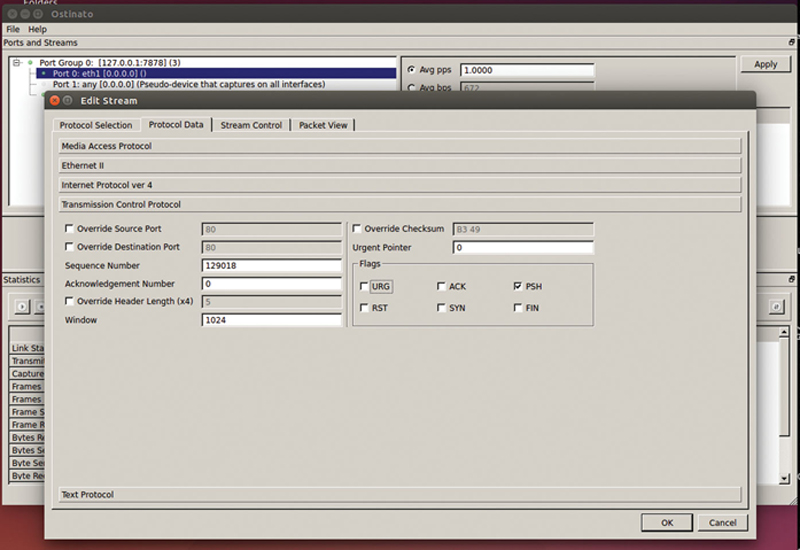
Figure 10.9 Layer 4 Header Editor Example.
The “Protocol Data” tab is meant to configure fields for layer 4 (Fig. 10.9). Here, we see TCP header (stateless) options. These can override the TCP destination port, TCP source port, L4 checksum, and length. In addition, they can provide static values for Sequence number, windows, ACK number, and urgent pointer. Lastly, the user can set TCP flags. As a best effort, set the PSH flag to tell the device under test to forward the segment as soon as possible.
Under the “Text Protocol” the user can perform Layer 5 actions like an HTTP get. In this example, the stream is issuing a GET method over HTTP 1.0 (Fig. 10.10).
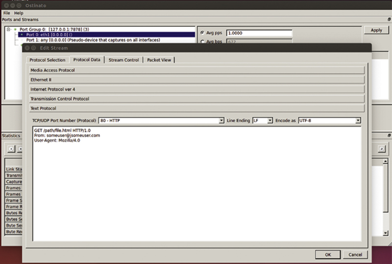
Figure 10.10 Upper Protocol Payload Example.
The next section is “Stream Control.” Here you can send packets or bursts of packets. When packets are selected, you can set the frame rate “Packets/Second” and the frame count. When in Burst Mode, you can set the total number of bursts, packets per burst, and the number of bursts per second. The rate and Interburst gap (IBG) will automatically be calculated. Lastly, after this stream finishes, you can choose a next option of stopping traffic, going to the next stream, or looping back to the first stream (Fig. 10.11).
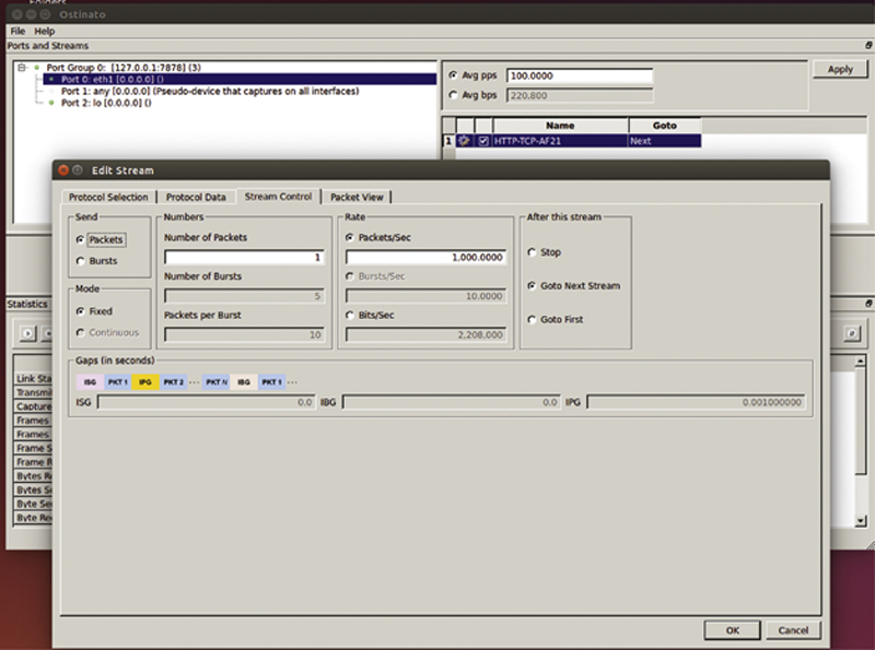
Figure 10.11 Stream Rate Control.
Finally, under packet view, you see a tree of what will be generated with the corresponding HEX and ASCII views (Fig. 10.12).
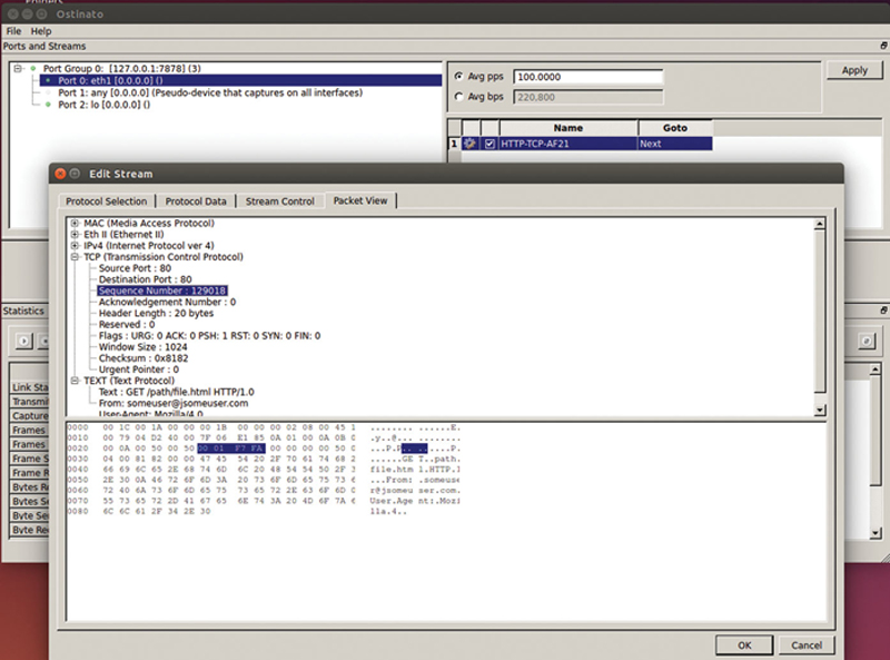
Figure 10.12 Packet View Similar to Wireshark.
When everything looks right, click OK. Now, add each of your streams you previously identified. When you are done adding Streams, be sure to hit “Apply” to commit the changes. Note, you can right click on a stream and save/load it to a file for archiving purposes.
In the main GUI, the “Statics and Control” section below allows you to see port level events. Ports represent columns, metrics represent rows. The port name “Port x-y” indicates port group “x,” and port “y.” To perform an action on a port including starting and stopping traffic, clearing traffic results and starting and stopping capture, you need to click on the column header to select the entire column. Note, you can shift-click to control multiple ports at the same time.
The first control button starts traffic on the selected ports, the button next to it stops traffic. The “Lightning” Button clears results of the selected columns, whereas the “Lightning-page” icon next to it clears all results globally. The next icon starts capture on separate ports (Note if start capture on the “any” port, you can capture on all interfaces at the same time) (Fig. 10.13).
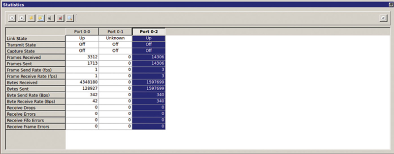
Figure 10.13 Counter Windows.
The icons next to it will stop capture and then view in Wireshark. Note, you can tear off the statics window if you want to place it on a different monitor and you can File > Save or File > Open your entire test config. If you click icon to the far right, you can remove ports from the statics window view and clicking the multiwindow icon in a town off stats window will redock it back to the tool.
In addition to using the GUI, you can also build and drive traffic through Python. To install support for scripting, ensure you have python installed by typing:
sudo apt-get install python
sudo apt-get install python-pip python-dev build-essential
sudo pip install --upgrade pip
sudo pip install --upgrade virtualenv
Next, you need to install support for Ostinato for Python by typing:
pip install python-ostinato
A good reference for automating Ostinato with Python is located at https://github.com/pstavirs/ostinato/wiki/PythonScripting.
Testing TCP with iPerf3
iPerf3 is a testing too that allows you to test Layer 4 transport performance, specifically focused around stateful TCP. You can think of iPerf as having a traffic generator feeding a stable TCP connection. This is both useful and cautionary, in the fact that you have traffic that will measure the impact of network impairments like packet loss, jitter, and latency. From a cautionary perspective, raw TCP traffic has a lowered degree of realism because the Layer 5-7 portion of the tool is not a true upper layer protocol. So what you are testing looks more like a large transfer FTP as opposed to HTTP, which tends to be bursty. As with all tools, know the benefits and limits and understand what you are really testing.
First, we have to install iper3 on Ubuntu Linux. To do this, open up a terminal window and type the following:
sudo add-apt-repository “ppa:patrickdk/general-lucid”
sudo apt-get update
sudo apt-get install iperf3
To verify iperf3 is installed, you can type the following:
iperf3 -v
When working with iperf3, you need to identify and configure a TCP/UDP client and server. We will initially focus on TCP. Then, you need to determine how many concurrent sessions you want to load the SUT. Please note that there are no upper layer protocols, so if you go through a firewall, the only way the firewall will pass traffic is if you configure RAW or no upper layer protocol inspection (If it is looking for an HTTP information, it will not be present in the TCP traffic generated by iPerf3).
We need to first configure the TCP server. On the TCP server host, the base command to start iPref3 Server is
sudo iperf3 -s -p 80 -fm -V -i 1 -D -B127.0.0.1>TCPServer_Port80.txt
Here is the definition of the flags set in this example:
-s
Run instance of iPerf3 in Server Mode
-p 80
Listen on port 80.
-fm
Use Mbits as unit
-V
Display verbose mode information
-i 1
Display information every 1 second
-D
Run as a Daemon (Background Process)
-B127.0.0.1
Bind to the IP address (assigned to an interface) 127.0.0.1(localhost)
> TCPServer_Port80.txt
Redirect output to a file
It is also very useful to have multiple TCP listening ports in play at the same time (HTTP(80), HTTPS(443), FTP (20/21)). By using the “&” directive, you can place each in their own process.
To set up the TCP client, use the following example:
sudo iperf3 -c 127.0.0.1 -p 80 -fm -i 1 -V -d -b 500M -t 120 -w 64K -B127.0.0.1 -4 -S 0XB8 -p 1 -O 0 -T “MY Output”>TCPTestPort80.txt &
Here are what the client flags will set:
-c
Set this instance of iperf3 as Client
-p 80
Client will try to connect on port 80
-fm
Client will display rests as Mbits
-i 1
Client will output every 1 second result for TCP connections generated from this process
-V
Client will dump Verbose Mode data to stdout
-d
Client will dump debug data to stdout
-b 500M
Client will attempt to scale to a target of 500 Mbps per TCP connection, network impairments and client/server hardware/OS may limit this rate.
-t 120
Test for 120 seconds
-w 64K
Use a window size of 64 Kbytes
-B127.0.0.1
Bind the client to the interface configured to 127.0.0.1
-4
Use IPv4 (as opposed to IPv6)
-S 0XB8
Set the Client ToS/DSCP codepoint to specified value for each of the TCP connections
-p 1
Generate specified number of concurrent TCP connections to server (Partial Mesh). In this case 1.
-O 0
Omit the first “0” seconds of results. In this case show all results
-T “MY Output”
Write the string “MY Output to each row entry in the results.
> TCPTestPort80.txt
Output results to specified file
&
Run instance of iPerf3 client in its own process.
Now that we have described the mechanics of using iPerf3, we need to talk about best practices of generation and analysis. After identifying what will be tested (Firewall, IPS/IDP, Server), around the SUT with test end points. Notice too that there is no reason why a single interface cannot be both a client and a server port. When configuring a client, utilize the “-p” to create multiple concurrent connections. Add one instance of client per TCP server port and run them as different process in Linux using the “&” directive. Each process should have a unique out file name (eg, TCP_FTP_127.0.0.1_Port21). On the server side, set up one iperf3 instance per TCP listening port that you have identified in your network and run them each as daemons (“-D” flag). Now, if we combine this with a client side bash script to cycle through concurrent connections we can “Scan” to see what is the maximum number of open connections across a range of target bitrates.
When you look at the client results (Fig. 10.14):
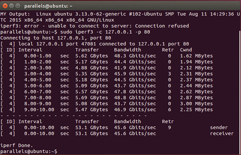
Figure 10.14 iPerf3 Interval Data Rates.
Here, we see rows represent a 1 second interval, the amount of data transferred in that Interval, the calculated bandwidth within that interval, number of retransmission and the Cwnd, which is the amount of data that is transferred before a ACK is sent. Also not the very direct column is the connection ID, when you specify multiple concurrent connections, they are uniquely identified by the ID. At the very end, you see a summary of all connections tested.
When you add the “-d -V” flags to the client, now you see one level down in results (Fig. 10.15).
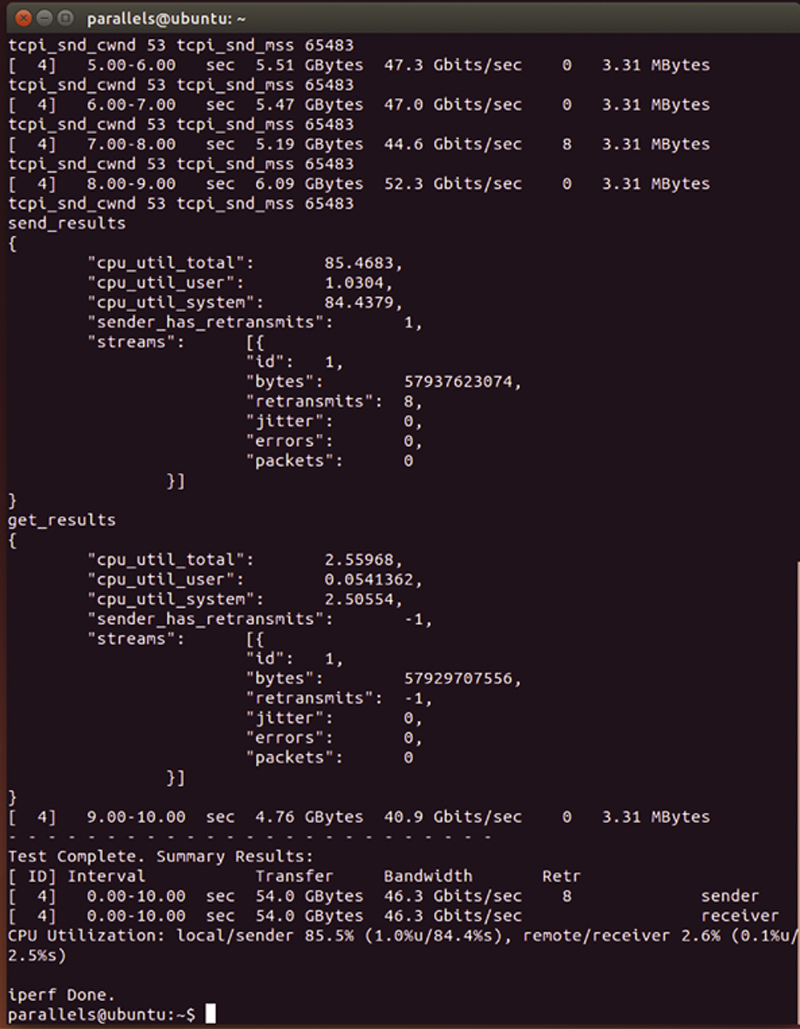
Figure 10.15 TCP Layer Error Event Counters.
Per TCP connection you will be show CPU utilization used. Further, you will see the number of retransmissions, errors are measured, and aggregate bandwidth. If you see retransmissions or errors, it is a good indication that the SUT is overloaded; you need to reduce the number of concurrent TCP connections and/or target bandwidth.
iPerf3 can also measure UDP performance, Here is an example:
iperf3 -c 127.0.0.1 -fm -b 1G -u -V -d
In this case the “-u” specified UDP and we will open Port 5201 (the default) and attempt a 1 Gbps transfer (Fig. 10.16).

Figure 10.16 TCP Summary Results.
What you want to look for here is errors and excessive PDV (Packet Delay variation, or Jitter). When either of these is high, you have to lower the UDP connection count and the desired transfer rate. Again, a bash script helps you scan through these.
In addition, iPerf3 allows the user to specify the TCP or UDP payload using the ‘-F {File Name}’ command line option. This allows you to write upper layer headers to get one layer deeper in the SUT (For example you can add an HTTP GET). The file source needs to be a text file. One line of the file will be grabbed and sent in order. On the server side, specifying the “-F {Fielname}” flag will record to disk the client side requests as opposed to discarding the requests. This is useful if you want to see how the SUT is modifying the client request in transit. There is no way to specify an equivalent server response.
iPerf3 takes the pathways that you previously tested and allows you to see the impact of network congestion, server side impairments, as well as how efficiently the target server can handle TCP connections. You should notice, for example, that if you have a server NIC that handles TCP offload, the CPU utilization should be substantially lower than if the CPU is fully processing the TCP connection. Also, given that a major source of poor quality of experience is an over subscribed server, using iper3 to measure the TCP impact takes you a step closer to rightsizing your server pools.
Using NTOP for Traffic Analysis
NTOP is a powerful multinode graphical analyzer of traffic across the network. The system is extensible through a plugin system, allowing for deeper analysis of the network. NTOP can be used in conjunction with traffic generators to analyze flows across the network. The first thing we have to do is install NTOP on Ubuntu Linux. To do this, open up a terminal window and type:
sudo apt-get install ntop -y
You will be asked for a monitor port (such as “eth1”), and a root NTOP password. After installation is complete, open up a web browser in Ubuntu and type:
http://localhost:3000
If you are asked, your username is “admin” and the password is the entry you typed.
The default view is Global Statics, here you can see the monitored ports. If you click on the Linux netlister log Report tab, you can see different distributions of unicast/multicast/broadcast, frame size distribution, and traffic load as a summary.
If you click on Protocol distribution you can see by IP version distribution of network transports. This should roughly match your test traffic generation. Note that if you generate streams with no upper layer protocols, the percent and bandwidth will show up under “Other IP”
Finally, if you click on Application Protocols, you can see a breakdown by protocols, starting with an eMIX distribution and followed by a historical load vs. time per protocol.
Note, if you click the magnifier icon to the right, you can drill into a protocol and change the time domain to examine bandwidth vs. time per protocol. If you use this in combination with TCPreplay, you can measure the performance of a stateful device like a firewall. If you compare Ingress rate to egress rate as a ratio, you can see the impact of the SUT on traffic.
Now the user has the option of looking at Summary, All Protocols, or by IP. Summary traffic will show the user aggregate traffic across the monitored interface. The hosts option will show the detected IP addresses in the traffic stream. This should match the traffic that was generated by your traffic (Fig. 10.17).
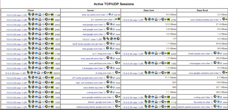
Figure 10.17 Live TCP/UDP Connections.
Here, if you compare what was the offered load to the network vs. the measured load, you can determine how the device is effecting traffic. Since this view is live, you should be able to modify the traffic bandwidth, connection count, or transaction count and see the effect.
In addition to basic network statics, you can also add some additions to nTop including nProbe and nDPI. There is a fee for this, but the return on investment includes deeper protocol analysis and distributed monitoring of test and live traffic. The link may be found here (http://www.ntop.org/products/netflow/nprobe/). There are three basic modes for nProbe. In Probe mode, nProbe acts as a netflow probe, taking in Netflow data and analyze it. To start in probe mode, type:
“nprobe -i eth0 -n collector_ip:2055”
In collector mode, you mirror live traffic to nProbe, and it will perform direct traffic analysis, saving flow data to an MySQL database. The command to launch nProbe in this mode is:
nprobe –nf-collector-port 2055
Finally, you can place the probe in Proxy Mode; this allows you to place the probe inline with traffic between a Netflow probe and a collector, so it can perform deep analysis of application traffic. The way you launch the probe in this mode is by typing:
nprobe –nf-collector-port 2055 -n collector_ip:2055 -V]
Lastly, you can extend nProbe by adding the protocols that make the most sense for your environment. The Store to find and purchase these plugin is here (http://www.nmon.net/shop/cart.php).
When you have a high speed network (1G or higher), you need to make sure you have the wire rate NIC driver (for purchase on this site). You will want to purchase a “PF_RING ZC” driver for each high speed NIC. This will give you wire rate performance. There are two basic models, a 1G and 10G NIC driver.
Applied Wireshark: Debugging and Characterizing TCP Connections
When you are analyzing TCP issues in the network, Wireshark is a very useful tool. When filtering captured traffic, find a packet contained within the TCP connection in question. Right-click the packet and select “Follow TCP.” This will narrow down the displayed content to the TCP connection in question. Now, if you launch IO graph, you can change the tick interval to 0.1 seconds at 5 pixels per tick. On the Y-axis you can change the unit to Bytes per Tick and the scale to Logarithmic. Now in the Graph 2 filter type in the following and change the graph type to FBar:
tcp.analysis.flags $$ !tcp.analysis.window_update
What this will do is graph TCP errors but exclude TCP window updates (while are good). When we overlay these onto the same graph we get Fig. 10.18.
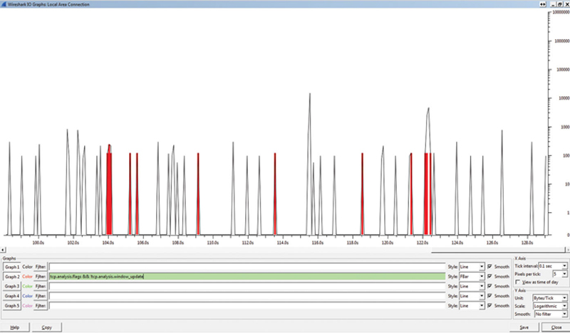
Figure 10.18 TCP Flag Events Over Time.
You can clearly see how the TCP bandwidth (black) is effected by TCP events (red bar). Thus, through visual inspection, we can assume a correlation. If you click on a red bar, that will take you to the error-based TCP packet. Here we see there is a ZeroWindow error (Fig. 10.19).
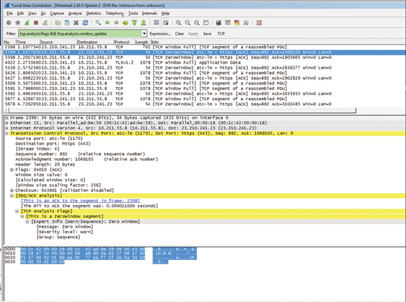
Figure 10.19 Dereference Effected TCP Packet.
The root cause of a ZeroWindow condition is the end node TCP stack is too slow to pull data from the receive buffer, and that Window scaling is either not on either side or not working, or being modified by the SUT.
In addition, you can find specific TCP errors by using the display filter “tcp.analysis.” This will show you a full list of events (Fig. 10.20).
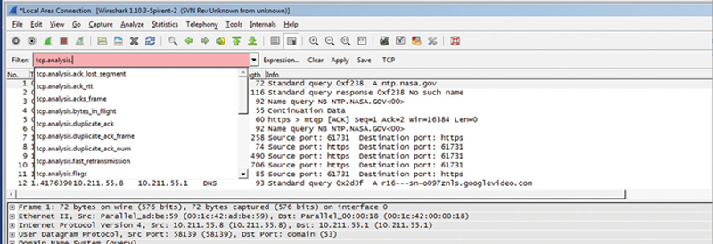
Figure 10.20 Example Wireshark Display Filter.
According to Wireshark’s Wiki (https://wiki.wireshark.org/TCP_Analyze_Sequence_Numbers), here is the meaning for each type of error:
TCP Retransmission—occurs when the sender retransmits a packet after the expiration of the acknowledgement.
TCP Fast Retransmission—occurs when the sender retransmits a packet before the expiration of the acknowledgement timer. Senders receive some packets that sequence number are bigger than the acknowledged packets. Senders should Fast Retransmit upon receipt of three duplicate ACKs.
TCP_Out-of-order—occurs when a packet is seen with a sequence number lower than the previously received packet on that connection.
TCP Previous segment lost—occurs when a packet arrives with a sequence number greater than the ”next expected sequence number” on that connection, indicating that one or more packets prior to the flagged packet did not arrive. This event is a good indicator of packet loss and will likely be accompanied by ”TCP Retransmission” events.
TCP_ACKed_lost_segment—an ACK is dropped in transit across the network.
TCP Keep-Alive—occurs when the sequence number is equal to the last byte of data in the previous packet. Used to elicit an ACK from the receiver.
TCP Keep-Alive ACK—self-explanatory. ACK packet sent in response to a ”keep-alive” packet.
TCP DupACK—occurs when the same ACK number is seen AND it is lower than the last byte of data sent by the sender. If the receiver detects a gap in the sequence numbers, it will generate a duplicate ACK for each subsequent packet it receives on that connection, until the missing packet is successfully received (retransmitted). A clear indication of dropped/missing packets.
TCP ZeroWindow—occurs when a receiver advertises a received window size of zero. This effectively tells the sender to stop sending because the receiver’s buffer is full. This indicates a resource issue on the receiver, as the application is not retrieving data from the TCP buffer in a timely manner.
TCP ZerowindowProbe—the sender is testing to see if the receiver’s zero window condition still exists by sending the next byte of data to elicit an ACK from the receiver. If the window is still zero, the sender will double his persist timer before probing again.
TCP ZeroWindowViolation—the sender has ignored the zero window condition of the receiver and sent additional bytes of data.
TCP WindowUpdate—this indicates that the segment was a pure WindowUpdate segment. A WindowUpdate occurs when the application on the receiving side has consumed already received data from the RX buffer causing the TCP layer to send a WindowUpdate to the other side to indicate that there is now more space available in the buffer. This condition is typically seen after a TCP ZeroWindow condition has just occurred. Once the application on the receiver retrieves data from the TCP buffer, thereby freeing up space, the receiver should notify the sender that the TCP ZeroWindow condition no longer exists by sending a TCP WindowUpdate that advertises the current window size.
TCP WindowFull—this flag is set on segments where the payload data in the segment will completely fill the RX buffer on the host on the other side of the TCP session. The sender, knowing that it has sent enough data to fill the last known RX window size, must now stop sending until at least some of the data is acknowledged (or until the acknowledgement timer for the oldest unacknowledged packet expires). This causes delays in the flow of data between the sender and the receiver and lowers throughput. When this event occurs, a ZeroWindow condition might occur on the other host and we might see TCP ZeroWindow segments coming back. Do note that this can occur even if no ZeroWindow condition is ever triggered. For example, if the TCP WindowSize is too small to accommodate a high end-to-end latency this will be indicated by TCP WindowFull and in that case there will not be any TCP ZeroWindow indications at all.
Emulating the Behavior of the WAN for Testing
When testing the network, it is important to consider the effect of the WAN on Quality of Experience. If you think of the connection between your users and the Server pool, you have a certain budget of tolerance that can be spent hopping across the network and still have an acceptable quality of experience. When testing, it is useful to be able to emulate the effects of the WAN, giving that sometimes upward of 90%+ of the budget tolerance cannot be avoided (latency in the ground going through an ISP). To emulate WAN condition in a controlled fashion, we will use WanEM (http://wanem.sourceforge.net/). WanEM is available as an ISO or an OVA/OVF format. WANEM may also be used in a virtual environment mapped to two vSwitches containing physical NICs. By definition, you will need two or more NICs on the WanEM Host.
After downloading the ISO image, either burn it to a DVD for booting or build a VM with two virtual NICS. When you get the “boot:” prompt, press enter. The tool will ask you if you want to configure the IP addresses using DHCP, say no. Follow the wizard to configure the IP addresses. You will be asked for a master password, which you should enter. Your login will be perc/{Your password}.
To get to the main screen, use a web browser and type:
http://{IP of the appliance}/WANem
Using impairment tools is conceptually very simple, you place the impairment appliance inline between your traffic generator emulating client and your server pool. The impairment tool is considered to be a “Bump in the wire” which means it does not route but stores, impairs, and forwards traffic to the other interface.
WanEM also allows you to configure your traffic impairments in each direction, if you choose. Initially, the tool is in “Simple Mode,” which means it is symmetric (all impairments apply to both directions) and you can only control basic impairments like latency and packet loss. Advanced mode allows you to rate shape the traffic, inject errors, and perform filtering on the traffic. The manual is very easy to understand, so I will not go over how to configure the tool, but instead give you WAN recommendations.
As a rule of thumb, every 100 KM of fiber will induce about 1 millisecond of latency. If you take the direct path from city to city you wish to emulate (Google is good for this) and multiply it by 1.3 (Wan links are never a single straight line, then divide by 100 KM, that will give you a good rule of thumb on how much static latency to inject in each direction. You can also assume latency PDV (jitter) will be ∼1% of this latency, so you can layer that on. Now, private WAN links should not experience drop, but if you are testing something like a VPN that goes over the Internet, a good worst case scenario is 3% packet loss. By emulating impairment, you are more likely to catch issues in the SUT, especially with TCP-based traffic.
Summary
The ability to stress test traffic over your network and measure the effect is a critical part of understanding the limits of your design. In this chapter, we used open source tools to test traffic and measure the performance across the network. In addition to understanding the limits of performance of the network, establishing a baseline is critical for future impact analysis when measuring the potential impact of performance attacks may have on the network.