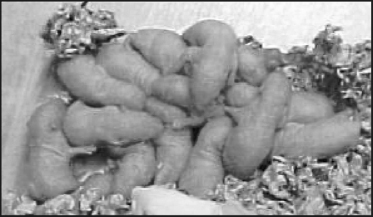
Figure 6.1
A huddle of two-day-old albino rat pups (Rattus norvegicus) with mother.
6
Models as Scaffolds for Understanding
The term model has a variety of context-dependent meanings. A common meaning of model is to represent a physical system. Examples of representational models include mathematical and computational models of populations, ecosystems, or traffic flows. Sometimes, a model is primarily used not representationally but rather as an instantiation of an idea such as robots that can interact with humans, computational agents that play games, or agents that search the Internet. Often the intended meaning is less clear. For example, the notion of model organisms is increasingly common in the biological sciences. A model organism in one sense is intended as a representation of, for example, some human disease condition, but model organisms are also investigated to better understand the model system itself. These and other senses of model are used every day in science, and their meaning differs primarily in the functions they serve. Models are therefore multifunctional, and whether they are representational is more or less important depending on the context of research. In this chapter, our primary focus is on models as representations of physical animate systems (e.g., animals) that support our understanding of those systems. It is in this sense that models are most closely connected to the idea of scaffolding as it is used in this anthology.
No model is a perfect representation of another physical system. If models are identical to a system represented, they are of no use (beyond observing and manipulating the system itself) because there are no differences between model and system. The main reason for building representational models is to build simpler representations that we can analyze, manipulate, and understand. There is a cost to simplification because not all characteristics of the modeled system are represented by a model. A model is always false as a representation of all or many properties of a system.
Simplification is not the only source of falsity in models. Ignorance of the system modeled is another. Many representational properties of a model do not correspond directly to properties of the system modeled because of our uncertainty about whether a system has the properties in question. For example, when a physical system is modeled mathematically, the mathematical properties of the model do not directly correspond to properties of the physical system. Instead, they correspond to mathematical properties of measurements taken of the system, and the measurements systems are themselves models of the data.1
In addition to simplification and ignorance, the properties of a model can make it an in principle false model as a representation of a physical system. Differential and partial differential systems of equations are often used to model biobehavioral systems, and yet such models assume inherently continuous systems, but populations or groups of individuals are not continuous. Physical models such as robots may not share the same physical properties as the system represented, and these differences often matter. Even highly technical assumptions matter. For example, in agent-based modeling, whether updating is synchronous or asynchronous matters (Caron-Lormier et al. 2007). Even when we are satisfied that a model’s properties correspond to system properties (e.g., the representation of population size in a differential equation), the correspondence is still strictly speaking false and at best heuristic.
How models are false matters (Wimsatt 1987). When models are false in ways that do not represent a system or fail to predict the behavior of a system, then they fail to support our understanding of the system. A good representational model—even if it is very simple—should predict, explain, or lead to some understanding of the mechanisms that produced the data. We must understand how assumptions are important or unimportant and in what contexts. These are fundamental problems of representational modeling, and there are no recipes for success.
We therefore knowingly build false models and we do so mainly for practical and epistemic reasons (e.g., analysis, manipulation, ignorance, building on previous models, accepted tradition, and limitations of the nature of the models to represent a system). The assumptions we make are a problem for scientific understanding because we need to (1) know which false assumptions matter and which do not, (2) make true statements about the system of interest if we are to understand it, (3) propose plausible mechanistic explanations, (4) formulate plausible hypotheses about a system, (5) identify problems and new directions for research, and (6) propose new models that are informed by our errors (Wimsatt 1987, 2007). These are essential for the scaffolding functions of models in science.
Richard Levins (1966) was well aware of the problem of false models in science. Levins provided a pragmatic framework for explaining both how and why models are false based on the practical impossibility of simultaneously maximizing truth along the dimensions of generality, realism, and precision. Levins’s solution to the problem of false models is robustness analysis. If there are a number of models of a system and they make different assumptions, then understanding is based on robust elements of these models: “our truth is the intersection of independent lies.” There, however, have been disputes about Levins’s robustness analysis of false models (Orzack and Sober 1993; Levins 1993; Webb 2001 and commentaries therein; Odenbaugh 2006; Weisberg 2006).
We must, however, always keep in mind that robustness analysis is a heuristic strategy that can be systematically misleading. Robustness analysis, whether in its nonscientific logical sense (see Orzack and Sober 1993) or in a weaker pragmatic sense (see Weisberg 2006), assumes an unbiased representation of all (Orzack and Sober 1993) or some (Weisberg 2006) of the possible models of a system. In actual practice, we have no idea whether our models are a representative sample. In some cases, we may have a number of models that appear to be representative of the space of possible models but are instead a biased sample from some restricted region of model space. For example, Wade (1978) showed that a number of models of group selection made assumptions that largely ruled out group selection as an important force in evolution. He then showed that alternative assumptions, based on his experimental research, indicated that group selection could be an important force in evolutionary processes. Thus, Levins’s robustness is heuristic and can systematically break down. Robust models scaffold our understanding, but even robust models can be systematically misleading.
A more important strategy of model building than Levins’s robustness is Wimsatt’s (1987, 2007) strategy of error diagnosis. Models always fail to match data adequately in some respect, but these mismatches can serve to diagnose problems and build improved models. Wimsatt (1987, 2007) discussed examples of this use of model mismatches with the data and mechanisms in the development of our understanding of chromosomes. In identifying and diagnosing mismatches with both data and mechanisms, we are performing another scaffolding function of modeling in science. As we diagnose mismatches and build better models, we also build our understanding of the systems we are interested in.
Another strategy for using models, implied by Wimsatt’s (1987) error diagnosis, is to downplay the importance of the truth of a model. There are two functions of models that allow them to scaffold our understanding of systems without invoking truth. First, a model must produce relevant data or demonstrate that relevant data can be produced by the mechanism assumed in the model. Second, the data produced by a model must not only match data of the system but must also match relevant aspects of the mechanisms operating in the system (see Giere 1988 for a similar account). On this view, to support the understanding of a system, a model must (1) assume a mechanism for producing the data, (2) produce matches to the data produced by the system, and (3) match the mechanisms of the system in relevant respects. Once the quest for truth is abandoned in favor of focusing on production and matching, then the scaffolding function of models for understanding begins to makes sense even though the models we work with are false.
Experiments as Models
Models are not limited to mathematical and computational models. The vast majority of representational scientific models are physical models, and the most common physical models are experiments. Experiments can investigate how mechanisms work in a system (e.g., the causal role of a hormone such as a oxytocin in the social behavior of prairie voles; e.g., Carter 2003; or increased sharing in humans; e.g., Zak et al. 2007) or how one system is used to investigate another (e.g., drugs tested in animals for potential human use or animals used as models of human diseases).
Experiments share characteristics in common with mathematical and computational models. Most importantly, simplifying assumptions are made in the design and implementation of experiments. If we are investigating the role of a hormone in the behavioral mechanisms of rats, a variety of explicit and implicit simplifying assumptions are made in design and implementation of such experiments (e.g., the strain of laboratory rat, housing conditions, experimental apparatus, and measurement techniques). Just like mathematical and computational models, assumptions we make in experiments are often false, at least from an ecological perspective. For example, to return to the role of a hormone in the behavioral mechanisms of rats, the laboratory habitat is radically different and simpler than the natural habitat in many respects (e.g., elimination of predators and pathogens, constant availability of food and water, constraints on movement and social interactions), which could be highly relevant to the production and expression of hormones.
An important characteristic of experiments is that they involve producing and matching. Design, engineering, and construction go into building an experiment that produces data. For example, an experiment using rats includes a number of design and construction elements. Maintenance of animals requires the construction of housing environment. Testing apparatuses must be designed and built to produce data. How they are built matters (Timberlake and Lucas 1989). Protocols must be developed for executing the experiment and collecting data. All of these building activities and more go into constructing an experiment that will produce data. These design and construction activities are essential to experimentation because by carefully constructing an experiment we gain control and insight into how the experiment produced the data.
The next step is matching. Matching may be simple and crude. In null hypothesis testing,2 the theoretical hypothesis is that a specific manipulation (i.e., independent variable) produced changes in one or more response variables (i.e., dependent variables). The null hypothesis is that the data do not differ from the control condition in which the manipulation is not performed. If the data are significantly improbable assuming the null hypothesis, the null hypothesis is rejected in favor of the theoretical hypothesis. This is a crude form of matching at best (Cohen 1994). Even if we conclude, for example, that the hormone oxytocin affects social behavior in the laboratory, it may or many not do so in another context (e.g., naturalistic settings).
Scaffolds: How Experiments as Models Support Understanding
In experimentally driven areas of the biological and behavioral sciences, understanding how a system works is given by verbally describing its component mechanisms supported by experiments, which were conducted by various scientists at various places and times. Ovulation in mammals, for example, is a complex system that begins early in development with the origin of primordial germ cells in the ovaries and involves a number of complex transitions of germ cells to the ultimate stage of ovulation. In a recent review article “Understanding follicle growth in vivo,” Oktem and Urman (2010) described the follicle growth system and its mechanisms buttressed by various scientific experiments. We quote a small part of the beginning of their paper to illustrate how experiments are used to scaffold understanding in the experimentally driven sciences:
PGCs [primordial germ cells] first appear as a cluster of ~100 cells in the endoderm of the dorsal wall of the yolk sac near the allantois between the third and fourth weeks of gestation in the human (McKay [sic] et al. 1953). PGCs then migrate to the hindgut and dorsal mesentery during the fourth and fifth weeks of gestation, respectively (McKay [sic] et al. 1953). By the seventh week of gestation, colonization of gonadal tissue by germ cells is complete. Germ cells are essential for the formation and maintenance of the ovary: in their absence the gonad degenerates into cord-like structures (Merchant-Larios and Centeno 1981). Once the PGC [sic] have arrived in the gonad, they undergo more extensive proliferation such that their number rapidly increases from merely 10 000 at the sixth week of gestation to 600 000 at the eighth week. With rapid mitotic activity, their number further rises to 6 million at the 20th week of gestation; thereafter the rate of oogonial mitosis progressively declines and ends at ~28 weeks with an almost equally increasing rate of oogonial atresia, which peaks at 20 weeks of gestation... (Oktem and Urman 2010, 2944)
Notice that the description is given as a process and the full review articulates the mechanisms causally operating among components based on a number of experiments. The experiments cited were conducted on several species (e.g., mice, rats, sheep, humans) and conducted using a variety of experimental designs and physical setups. If we view these experiments as physical models of systems, then giving a mechanistic account of the process of ovulation in mammals appears to be based on a hodgepodge of experiments conducted on various species, at various times, and under various circumstances. How do we know that all of these experiments of the various components of a complex mechanism work together as supposed?
Compositional Coherence
Each experiment cited in the previous section produced data relevant to the mechanisms and processes of ovulation. These experiments were cited with the intention of providing particular demonstrations of components of causal mechanisms and processes involved in the developmental origin and process of ovulation. Their citations in the text are intended as scaffolding for building understanding about the complex mechanisms operating in the origin and process of ovulation. The problem is that the processes and mechanisms of ovulation, as expressed in the paragraph quoted above, are qualitative, particular, and verbal. The processes and mechanism of ovulation are based on a number of experiments conducted over time by different experimenters, using different methods, and with different species.
This is the problem of developing compositionally coherent mechanistic explanations based on particular experiments (Schank 1991). Experiments are highly particularized on a number of dimensions such as species, methods, techniques, and perspectives. They may support a coherent mechanistic account, but we do not know (Schank 1991). This points to the importance of developing mathematical or computational models to determine whether the verbal accounts of the mechanisms and processes cohere in a way that can produce data that matched empirical data (Schank 1991). This is another way in which models (in this case mathematical and computational models) can function as scaffolds for constructing coherent understanding from a collection of heterogeneous experiments (Schank 2000).
Phylogenies of Models and Scaffolding
Consider the Nicholson–Bailey model of host–parasite systems developed in the 1930s (Hassell 1978; Schank and Koehnle 2007). The original model was inherently unstable, leading to the extinction of host–parasite systems. The analysis of the Nicholson–Bailey model demonstrated that a simple model of host–parasite systems assumed could not produce the data observed in natural host–parasite systems. A number of subsequent models were developed and analyzed to explore the possible mechanisms for stabilizing host–parasite systems (see Hassell 1978 for a number of examples). Mistro, et al. (2009), for example, introduced a discrete lattice of patches, some configurations of which are host refuges. Hosts and parasites migrate from patches, and the Nicholson–Bailey model determines the dynamics within each patch. They showed that depending on the distribution of refuges, stability and instability can be produced and that spatial patterns of hosts and parasites can emerge, which are data that can be compared to empirical data.
These models form a phylogeny of models, which organizes their relationship to each other and how they were developed (Schank and Koehnle 2007). Merely showing that models can have a phylogenetic structure does not explain why model phylogenies emerge in science. After all, models do not evolve by mutation and selection. We hypothesize that they develop for two practical reasons. First, we typically start with relatively simple models and only work our way to different variations or more complex models as required to gain insight and understanding of a system. If problems are generated in the original model (e.g., the instability of the Nicholson–Bailey model), then it is good modeling strategy to build models with different mechanisms. Second, we are interested in theoretically understanding a system. In Nicholson–Bailey models, the development of understanding has focused on the mechanisms that produce stable host–parasite systems, which better matches data observed in nature and the laboratory (Schank and Koehnle 2007). We suggest that models, which function as scaffolds to understanding, will take the form of phylogenetic trees, where different branches on the tree buttress our understanding through robustness analysis across the branches. Some branches grow and others wither depending on the success of the models.
Building and Rebuilding Scaffolding for Understanding Aggregation in Rat Pups
In 1994, one of us (Jeff Schank) became interested in modeling the behavior of rat pups in huddles. Previous experimental research by Alberts (1978a, b; 1984) had shown that huddling by rat pups could explain group thermoregulation and energy conservation (Alberts 1978b; figure 6.1 illustrates a huddle of rat pups). Pups are three-dimensional, with appendages, and squirm in and out of the huddle. They produce heat, which is conducted to and from other pups and the environment. To model pup aggregation, simplifying assumptions had to be made. Simplification often requires transforming the initial problem into a simpler problem that is easier to model. In this case, a radical transformation was made from understanding group thermoregulation to understanding pup aggregation on a 2-D arena surface. In this section, we will illustrate some of the scaffolding functions described above for our ongoing research aimed at understanding aggregation in infant Norway rat pups.
Figure 6.1
A huddle of two-day-old albino rat pups (Rattus norvegicus) with mother.
First Laboratory Model
For reasons of tractability and out of ignorance, we began by transforming the problem of modeling group–behavioral thermoregulation in rat pups into a simpler problem of aggregation on a flat and level surface (Schank and Alberts 1997). Until about ten days of age (Schank 2008), rat pups cannot lift their bodies off the floor of an arena (though this differs by strain; Schank 2008). This allowed us to build an experimental model, which permitted a 2-D analysis of the dynamics of aggregation.
By restricting the original problem to one of aggregation and designing an experimental setup for producing aggregation, the first thing we noticed was that various patterns of aggregates of pups formed on the arena surface. We initially classified these patterns by the number of pups in each aggregate and called them aggregons (figure 6.2). We assigned an aggregation index to them by ranking them according to the largest aggregon and then the next largest and so on (figure 6.2; Schank and Alberts 1997). The higher the aggregon number, the more aggregated the pups were. This metric was also a model of the data.3
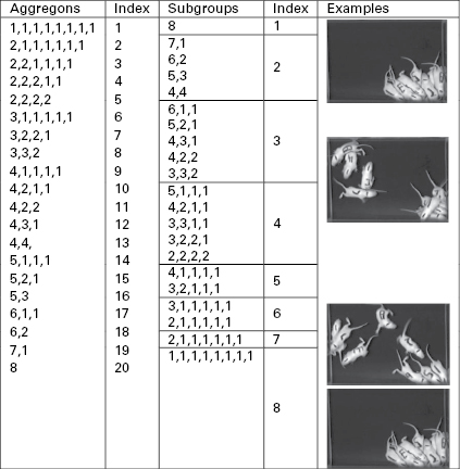
Figure 6.2
An illustration of our aggregation metric models. In the right column are pictures of pups in the arena, which illustrate each of our measures. The first two columns are aggregon patterns and their ranking for the degree of aggregation with higher indices indicating greater aggregation. The next two columns are subgroup patterns, and lower indices indicate higher aggregation.
Our transformation of the initial problem into a problem of 2-D aggregation in an arena involved a number of other assumptions (Schank and Alberts 1997). Although pups are born blind and deaf and remain so until about day 13, they have limited olfactory capabilities, they can detect warmth and contact, they exhibit taxic responses (i.e., oriented responses to external stimuli) to inclines, and negative phototaxic responses to light. Since we were primarily interested in how contact influenced aggregation, other factors had to be controlled (i.e., simplifications of holding conditions constant and/or randomization) by the experimental apparatus4 and procedures (Schank and Alberts 1997). Here are some of the factors we explicitly controlled: to control for (1) the effect of inclines, the surface of the arena was carefully leveled; (2) odors, the surface of the arena was cleaned with alcohol after each run; (3) temperature effects, chambers were built that controlled the ambient and surface temperatures and maintained them at near thermal neutrality; and (4) initial conditions, pups were placed in stalls facing in random directions.
The experiments we designed, built, and executed produced two kinds of data: aggregon patterns and patterns of activity. By controlling various factors affecting aggregation, we knew physical contact among pups was of primary importance. However, we knew little about how contact produced the patterns of aggregation we observed, so we developed an initial agent-based model to explore more precisely how these data could be produced by pup preferences for contact.
The First Agent-Based Model
The first model assumed that pups occupied discrete locations (cells) and no two pups could occupy the same location, both false assumptions.5 Body shape was not represented. The outer cells were “walls,” and the inner cells of the model arena were “empty.” A model pup could move one cell at a time, and the probability of moving to another cell depended on the pup’s orientation and whether the cell was empty, contained another pup, or was a wall (Schank and Alberts 1997).
Modeling activity with conditional probabilities permitted the derivation of analytical results that were useful for finding the best-fit model of the data. Data on active and inactive pups were taken in discrete time steps Δt, but by considering the limiting case where Δt → 0, the rate of change in the frequency of active pups could be defined using a differential equation.6 This equation defined the “flow” of pups into and out of active and inactive states over time, and by integrating it, we obtained an equation for the probability that a pup is active at each time step.7 To find values for the activity transition probabilities from activity to inactivity and vice versa, a nonlinear curve-fitting algorithm (Press et al. 1992) was used to fit the derived activity equation to the activity data.8
Simulations revealed that the model produced data that were similar to the data produced by our experiments. The Kolmogorov–Smirnov test revealed that the distributions did not significantly differ from each other.9 The main discrepancy, however, was in the most aggregated states, which visually matched only moderately well. In the best-fit simulations, pups were much preferred to empty spaces and walls. The model was highly sensitive to preferences for empty spaces but much less sensitive to preferences for walls (Schank and Alberts 1997).
The first model produced data that matched empirical data reasonably well, which indicated that our model might capture aspects of the mechanisms of aggregation. The model, however, did not match higher states of aggregation as well as the lower states. If we were merely developing the models as a hypothesis test from a “Popperian” perspective, then strictly speaking, this first modeling attempt was a failure (i.e., resulted in the hypothesis’s being falsified). However, our goal was to develop initial insight and understanding into the problem of aggregation with the recognition that subsequent models would have to be modified, rebuilt, or inspired by what we discovered. Thus, our next step was to further our understanding by diagnosing the mismatches and readjusting our scaffolding via building a new model and running new experiments.
The Second-Generation Agent-Based Model
After achieving some success with the first model applied to data from seven-day-old pups, we collected data on ten-day-old pups and applied the same model. It did not produce data that matched the data produced by ten-day-old pups. This suggested that an important component of the mechanism of aggregation was missing from the first model. After observing a number of ten-day-old pups aggregate, we noticed that after a while aggregates would synchronously become quiescent or active. This suggested to us that in ten-day-old pups, activity had become coupled to the activity of other pups they contacted (Schank and Alberts 2000).
To model coupled activity, the transitional probabilities from activity to inactivity and vice versa were reformulated as a function of the number of active and inactive pups a given pup contacted.10 The difficulty with modeling coupled activity is that it introduced more parameters, which increased the difficulty of matching data produced by ten-day-old pups with data produced by the model by brute force.11
To get around the parameter space problem, we used a simulated annealing algorithm to find models that matched the data.12 This required developing a fitness function model, which allowed comparison between model and experimental data.13 Using the subgroup measure (figure 6.2) and by modeling activity as coupled by contact, the extended agent-based model matched the data produced by our ten-day-old pup experiments (Schank and Alberts 2000). The patterns of activity were also matched (Schank and Alberts 2000). We interpreted the emergence of coupled activity in ten-day-old pups as an indication of the developmental emergence of sociality in rats since altering activity in response to others is a minimal condition for social behavior.14 This was an unintended consequence of the original modeling project. We did not initially set out to understand the developmental emergence of sociality in rat pups, but our experiments and models produced this insight. The latter result illustrates a kind of gain of capacity in the model—to generate unintended understanding—without having to model sociality explicitly: the model gains a capacity not explicitly “represented.”
Rat Pups and Robots
In 2001, Sanjay Joshi was interested in starting a bioinspired autonomous robotic research program which went beyond merely bioinspired. He was interested in establishing a collaboration in which autonomous robots would model a specific animal system and the building and development of autonomous robots would both be informed by empirical research and provide theoretical insight into the animal systems. Searching the University of California, Davis, faculty web pages, he found Jeff Schank and proposed that they develop such a research project using Norway rat pups.
In the meantime, Jeff Schank, at UC Davis, and Jeff Alberts, at Indiana University, had decided to continue their collaboration, and they deemed it important to work with identical testing apparatuses so that data produced by both labs would be empirically consistent. Thus, Jeff Schank worked with Dwight Hector (instrument designer, Department of Psychology) to develop two testing chambers that would allow greater control over various factors affecting pup behavior.15 This apparatus was used to run all pup experiments described below.
The autonomous robotic modeling approach was to develop both robotic and simulated robotic models (Joshi and Schank 2003; Joshi et al. 2004; Schank et al. 2004; Bish et al. 2007; May and Schank 2009; May et al. 2011). The first physical robot had two main features: first it was crudely shaped to resemble the body morphology of a rat pup, and second it had a contact sensor on the front, which allowed it to respond to object contact by turning (the response was programmable; see figure 6.3). The first-generation robot (figure 6.3 left) behaved qualitatively in some respects like a single rat pup moving in an arena. It tended to follow walls and to get “stuck” in corners, but not permanently (Joshi et al. 2004).16
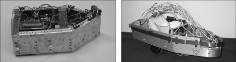
Figure 6.3
Pictures of the first-generation robot (left) and the second-generation robot designed to represent more accurately the body shape of a rat pup and to implement contact sensory all around the body (right).
The second-generation robot was scaled four times larger than a rat pup and had the body shape of a pup (cf. figures 6.1 and 6.3, right). We began testing the second-generation robots by implementing a subsumption-style behavior-based cognitive architecture.17 Movement was deterministic, but a few of the experimental runs yielded surprising results.18 Typically, a robot circled the arena repeatedly, but occasionally it did not.19 Rat pups behaved considerably differently than robots, instead of moving to one or more corners and apparently getting “stuck.”20 Occasionally, pups moved all over the arena,21 which resembled the anomalous robotic behavior in that both the robots and pups appeared to “bounce” off the arena walls very roughly analogous to billiard balls.22 This type of behavior is commonly seen in another strain of rat with a mutation in the vasopressin gene rendering it nearly nonfunctional (Schank 2009).
Jeff Schank subsequently attempted to implement the probabilistic movement and preferences for contact from the second-generation agent-based model. This implementation was a simplified version in which probabilities of movement were a function of contact only since robot sensors were not capable of distinguishing a wall from another robot. To our surprise, the robots behaved remarkably like rat pups upon visual inspection.23 Chris May, however, noticed that some of the Java methods used to program the robots did not behave as documented in the programming manual for the Parallax 25 MHz Java stamp 24-pin DIP module. The robots were essentially moving randomly, and preferences for contact were playing virtually no role in robot behavior!
We then decided that it was important to investigate the role of random movement in the aggregation of robots.24 After all, robots moving randomly due to programming errors looked very much like rat pups (all of our personal observations). Our implementation of random movement was similar to Brownian movement except that robots probabilistically backed out of corners.25 This was a “fix” to prevent robots from becoming “stuck” in corners.
When we ran simulation experiments in which we released a “litter” of eight robots in the arena, visually their behavior appeared remarkably like that of rat pups (see figure 6.4; May et al. 2006). Statistical comparisons revealed that the robots behaved similarly to rat pups on a number of metrics (May et al. 2006).26 These results suggested that random movement played a larger role in pup movement and aggregation than we had thought. The results also showed the importance of modeling body morphology, as mechanical interactions between robots and the arena created physical constraints on motion that allowed us to observe group patterns. One problem with this interpretation, however, was that there was a clear mismatch in mechanism at the level of morphology between rat pups and robots. As is apparent from figure 6.4, rats can flex their bodies whereas robots cannot because they are rigid.
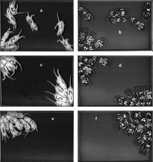
Figure 6.4
Examples of aggregation patterns of rat pups and robots in arenas. Day-7 pups (a) and robots (b) shortly after they are released or started. Day-7 pups (c) and robots (d) forming a subgroup that is not in a corner. Day-7 pups (e) and robots (f) aggregating in a single corner.
Simulating Rat Pups and Robots: Blurring Boundaries with Body Shape
The issue of rigid-bodied robots that could produce behavior similar to that of rat pups by moving randomly conflicted with previous agent-based models (Schank and Alberts 1997, 2000), which indicated that both object preferences and coupled activity are important for the formation of aggregates of rat pups on the surface of an arena. The robot results suggested that sensory processing might play a relatively small role in early rat development. This result was also in conflict with experimental results on the sensory capacities of developing rat pups (Alberts 1984). The need for modeling rat bodies extended in space was clearly important, but the assumption of rigid bodies, implicit in the construction of the robots, was clearly a false assumption that could matter.
The issue, as Chris May formulated it, became one of simulating parameters of body morphology to investigate how flexibility (passive and active) changed the behavior of robots. This was a critical step illustrating the use of models as scaffolds to understanding by diagnosing mismatches of mechanisms. The introduction of robotic agents as models of rat pups unexpectedly introduced the importance of body shape and flexibility in understanding pup aggregation. This led to a completely new line of model development—a branching in the phylogeny—focusing on the role of body shape and its interaction with the environment and other pups.
The body flexibility results were somewhat surprising.27 We had expected that increasing the realism of the model by introducing degrees of flexibility would have produced either a monotonically increasing or decreasing fit to the data, but it did not. Two-segmented agents produced the worst fit and three-segmented agents produced the best fit, but only to seven-day-old pups. The rigid body agents aggregated even less than the seven-day-old pups. Moreover, none of the agents came close to aggregating like ten-day-old pups. Three-segmented agents, which more realistically represent the flexible morphology of a rat pup, did result in the best match of all the body morphology models (May and Schank 2009; May et al. 2011).
Interestingly, while the rigid-bodied robots aggregated at intermediate levels between the two age groups of pups (May et al. 2006), the simulated rigid-bodied robots did not (May et al. 2011). This suggests that our physical sensors did matter for the robots and that the additional friction and snagging may have increased aggregation (see figures 6.3 and 6.4). This introduced a new mismatch between physical and simulated robots, which we have yet to resolve.
Third-Generation Agent-Based Model
Jeff Schank became intrigued by how the distribution of random movements in an arena affected both simulated robot group and individual behavior. Could movement in pups be modeled using two components of movement? The first was a matrix characterizing the probabilities of moving in random directions, and the second was a contact-based preference matrix. The two matrices were combined by multiplying (not matrix multiplication) the values of corresponding elements for both matrices and renormalizing to create probabilities of movement in different directions. Thus, the third-generation model differed from the second-generation model by explicitly incorporating different patterns of random movement (Schank 2008).
The resulting model was more complicated than the first two generations of models. To analyze this model, a genetic algorithm was used to find the best-fit models (Schank 2008). Ten models were evolved, all with similar but not identical parameter values (Schank 2008). The evolved models matched data on subgroup formation and wall contact especially well for seven-day-old pups and reasonably well for ten-day-old pups. Seven-day-old pups had random matrices in which pups moved forward less than the 2% of the time but moved back to left or right nearly 55% of the time. This produced “punting behavior” characteristic of rat pups at seven days of age (Alberts et al. 2004). The same random matrices also worked in group and individual contexts for seven-day-old pups, but not for ten-day-old pups.
The random matrices for ten-day-old pups changed as a function of social condition. In the context of a litter, the predominant direction of movement was straight ahead 36% of the time; otherwise, they tended to move either laterally or back-laterally 59% of the time. In sharp contrast, when ten-day-old pups were alone, they tended to move forward only 5% of the time and laterally 63% of the time (Schank 2008). These patterns of movement found in seven- and ten-day-old rats fit well with previous work, which showed that the spinal cord and neocortex of developing rats begin to connect at day 7 (see Schank 2008 for references and discussion). Thus, at seven days of age, random movement is stereotyped and does not vary as a function of social context, but by day 10—when the corticospinal tract is more fully developed—random movement becomes context dependent, providing a neurophysiological foundation for context dependent behavior in ten-day-old rats.
Discussion
The initial problem of rat-pup aggregation was aimed at understanding how rat pups huddle to thermoregulate and conserve energy. This was a hard problem to model, so we decided to transform the problem into a simpler problem that we believed would eventually lead to increased understanding of aggregation and eventually of the original problem. Even with an apparently simpler problem, building understanding of rat-pup aggregation was far from straightforward and did not resembled Popper’s (1963) “trial-and-error” approach to theory testing in which theories are arbitrarily generated and subjected to stringent falsification. Instead, our goal, as is typical of scientific modeling, was (1) to develop models that matched the data and (2) to do so by diagnosing problems in previous models to build better models.
Initially, we built two simple agent-based models to investigate rat-pup aggregation together with testing apparatuses and metrics for measuring aggregation. The use of robotic models introduced both initial confusion and insight. The initial confusion stemmed from random-robotic experiments that indicated that randomly moving robots behaved in similar ways to rat pups. These random robots used no cognitive rules (other than random movement), and they utilized no sensory information. Yet, we knew from past experimental work that this conflicted with what we knew about rat pups (e.g., Alberts 1984). Rat pups early in life have extremely limited sensorimotor capabilities, but they still do have them. Thus, the mechanisms did not match, but the data were disturbingly similar.
The initial confusion also led to insight and, we believe, understanding. First, analyzing how robots aggregated while moving randomly revealed that (1) body morphology and environmental structure were important for aggregation and (2) false assumptions (such as rigid bodies) could nevertheless produce data that matched pup aggregation while largely mismatching the underlying mechanism. Second, body morphology and kinematics required more investigation because some features of movement were robustly present across different body morphologies (i.e., asymmetrical corner contact; May and Schank 2009). Third, random movement is important. This was demonstrated by two radically different models on different branches of our model phylogeny (see figure 6.5). The first was the third-generation agent-based model, which used genetic algorithms to find movement matrices incorporating random probabilities of moving in given directions (Schank 2008). These probability matrices changed with age and neural development. We also found, when simulating robots with rigid and flexible body morphologies, patterns of random movement mattered for aggregation and unexpected but diagnosable mismatches occurred between simulated and physical robots (May and Schank 2009; May et al. 2011).
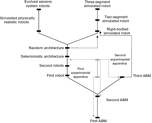
Figure 6.5
Phylogenetic trees of models. Solid black lines indicate lines of descent of simulation and robotic models. The solid blue line indicates the simple lineage of experiments. Green bars indicate different simulation and robotic models, and blue bars indicate experiments demarcated by experimental apparatuses associated with them. Dashed blue lines with arrows indicate data from experiments used to match models. Dashed black lines indicate data from simulations and robots used to match other models. At the base of the tree is the first agent-based model (ABM) (Schank and Alberts 1997), followed by the second ABM (Schank and Alberts 2000). The tree then branches. The right side is the third ABM (Schank 2009). The left side begins the robotic model phylogeny with the first robot (Joshi and Schank 2003; Joshi et al. 2004) and the second generation of robots followed by the deterministic and random cognitive architectures (Schank et al. 2004; May et al. 2006). The tree then branches again into two simulated robotic branches. On the left is the highly physically realistic simulated robot (Bish et al. 2007) followed by evolved sensory systems for these robots (Sullivan et al. 2012; not discussed in the chapter). The right branch introduces the simulated rigid, two-segmented, and three-segmented simulated robots (May and Schank 2009; May et al. 2011).
The use of scaffolding here differs in some important respects from its function in supporting a physical building or guiding education. Scaffolding that functions to support a building is constructed with a plan that is based on the plan for the building. This does not mean that scaffolding might not have to be rebuilt due to unforeseen problems, but generally, it is built with a plan. The way that models provide scaffolding for our understanding is also initially planned, but subsequent layers of scaffolding are built on previous layers, which is not necessarily part of the original plan (see Berryman, 1992, for a similar analysis for the origins of predator-prey theory). Models as scaffolds for understanding may have to be torn down or altered depending on what the models produce and how they match the data. The construction of new scaffolding depends on the insights and problems from previous models. Moreover, unlike a building, which, when constructed, provides its own support, our understanding cannot stand on its own and always requires scaffolding to hold it up.
In education, it is assumed that scaffolding materials and mentors support learning, and once learning is achieved, the scaffolding can be removed: the skills individuals acquire can then be practiced autonomously from the scaffold. In education, it is also assumed that scaffolding can be erected with a plan, a plan that might require adjustment for different children with different needs and in different cultural contexts, but it still is planned. For scientific understanding, however, research plans quickly go out the window. It is not that scientists do not plan their research; it is just that new results alter previous plans or initiate new and unexpected research directions. The process of building models as scaffolds for understanding in science is more a developmental than a planned architectural or educational process.
The model of scaffolding articulated here also illustrates how messy and piecemeal science is. Wimsatt (2007) articulated this issue well in his recent book Re-Engineering Philosophy for Limited Beings: Piecewise Approximations to Reality and in papers he has written over the last forty years. We do not know where a scientific problem will take us. We do not know whether a problem will be transformed into another. We typically make piecewise progress, which sometimes falls apart. We have also learned from Bill Wimsatt that we must use multiple methods and approaches. We do not believe that a single modeling approach is adequate. In our research program, we believe that the use of different kinds of models increased our understanding of rat-pup aggregation, but we do not know how many more models (including experiments with pups) we will build and execute before we can say we understand rat-pup aggregation, much less huddling, group thermoregulation, and energy conservation.
Notes
1. Suppes (1962) made a similar point more formally, namely, that there is a hierarchy of models from experiment to data to the match of data to models. From a practical point of view, there is not a hierarchy of axiomatized theories as Suppes’s analysis supposes. Instead, there is understanding based on prior experience, tradition, and semi-formal work on mathematical and computational models of data.
2. See Cohen (1994) for a critique of null hypothesis testing, which is the most commonly used method for matching data to hypotheses in the biological and behavioral sciences.
3. Later, we introduced a simpler index (Schank and Alberts 2000), which measured the number of subgroups of pups that formed (figure 6.2).
4. See Schank and Alberts (1997, figure 1) for an illustration of the first pup arena.
5. Figure 5 in Schank and Alberts (1997) illustrates the model pups and arena.
6. See equation 2, Schank and Alberts (1997).
7. See equation 3, Schank and Alberts (1997).
8. See figure 6 in Schank and Alberts (1997) for a comparison of the activity data and best-fit simulation distributions.
9. See figure 8 in Schank and Alberts (1997) for a comparison of the aggregon data and best-fit simulation distributions, p = 0.131 > 0.05.
10. See equations 5 and 6 in Schank and Alberts (2000).
11. It is often viewed as common knowledge that the more parameters a model has, the easier it is to fit the model to the data. This likely comes from statistical curve fitting, where, for example, the more parameters in a polynomial equation, the more complex curves can be fit. An extreme example of the failure of this commonsense knowledge is a linear model. No matter how many terms are added to a linear model, it still cannot fit a curve. In general, mechanistic models, as discussed here, will have rough data fitness landscapes, and the more parameters included, the rougher the landscape can become.
12. Simulated annealing was inspired by annealing in metallurgy (Kirkpatrick et al. 1983).
13. See equation 7 in Schank and Alberts (2000) for a more detailed discussion of fitness functions.
14. See figures 5 and 6 in Schank and Alberts (2000) for the degree of match between model and empirical data using simulated annealing.
15. See Alberts et al. (2004), figure 2, for the new experimental apparatus built based on the initial apparatus used in Schank and Alberts (1997), figure 1.
16. To avoid getting “stuck” in a corner, the robot was programmed to back up and randomly turn. This was a false assumption (rat pups tend to get stuck in corners, but they leave a corner typically by turning their head and moving along a wall, personal observation by Jeff Schank). By allowing the robot to back up and turn, the data were more similar to rat pups but the mechanism of turning failed to match.
17. A subsumption architecture is an approach to decomposing complex behavior into more simple modules that are organized into layers. Each layer implements a specific behavioral strategy, where higher layers are more abstract. An illustration of our simple architecture is illustrated in figure 7 in Schank et al. (2004).
18. See figure 8 in Schank et al. (2004).
19. Cf. figure 13a with 13b in Schank et al. (2004).
20. See figure 8b in Schank et al. (2004).
21. See figure 8d in Schank et al. (2004).
22. Cf. figure 8d with figure 13b in Schank et al. (2004).
23. This was unexpected because pup preferences for pups were much greater than for walls. Thus, because the robots could not distinguish other robots from walls, a good fit was not expected by directly basing preferences on the previous agent-based models.
24. The errors in the first programs for the robots introduced a new problem: how could robots moving randomly behave like rat pups? This is a simple illustration of how a false model—in this case a model with an unintended representation—can lead to new problems and insights.
25. See figure 8 in May et al. (2006).
26. For example, as illustrated in figure 10 (May et al. 2006), robots formed subgroups and contacted walls at levels intermediate between seven- and ten-day-old pups.
27. See figure 8 in May et al. (2011).
References
Alberts, J. R. 1978a. Huddling by rat pups: Multisensory control of contact behavior. Journal of Comparative and Physiological Psychology 92:220–230.
Alberts, J. R. 1978b. Huddling by rat pups: Group behavioral mechanisms of temperature regulation and energy conservation. Journal of Comparative and Physiological Psychology 92:231–245.
Alberts, J. R. 1984. Sensory Perceptual Development in the Norway Rat: A View toward Comparative Studies. In Comparative Perspectives on Memory Development, edited by R. Kail and N. Spear, 65–101. New York: Plenum.
Alberts, J. R., B. M. Motz, and J. C. Schank. 2004. Positive geotaxis in infant rats (Rattus norvegicus): A natural behavior and a historical correction. Journal of Comparative Psychology 118:123–132.
Berryman, A. A. 1992. The origins and evolution of predator–prey theory. Ecology 73:1530–1535.
Bish, R., S. S. Joshi, J. C. Schank, and J. Wexler. 2007. Mathematical modeling and computer simulation of a robotic rat pup. Mathematical and Computer Modelling 54:981–1000.
Caron-Lormier, G., R. W. Humphry, D. A. Bohan, C. Hawes, and P. Thorbek. 2007. Asynchronous and synchronous updating in individual-based models. Ecological Modelling 212:522–527.
Carter, C. S. 2003. Developmental consequences of oxytocin. Physiology & Behavior 79:383–397.
Cohen, J. 1994. The Earth is round (p <. 05). American Psychologist 49:997–1003.
Giere, R. N. 1988. Explaining Science: A Cognitive Approach. Chicago: University of Chicago Press.
Hassell, M. P. 1978. The Dynamics of Arthropod Predator–Prey Systems. Princeton: Princeton University Press.
Joshi, S. S., and J. C. Schank. 2003. Of Rats and Robots: A New Biorobotics Study of Norway Rat Pups. In Proceedings of the 2nd International Workshop on the Mathematics and Algorithms of Social Insects, edited by A. Carl and T. Balch, 68–74. Atlanta: Georgia Institute of Technology.
Joshi, S. S., J. C. Schank, N. Giannini, L. Hargreaves, and R. Bish. 2004. Development of autonomous robotics technology for the study of rat pups. Proceedings, 3:2860–2864. Washington, DC: IEEE Computer Society Press.
Kirkpatrick, S., C. D. Gelatt, and M. P. Vecchi. 1983. Optimization by simulated annealing. Science 220: 671–680.
Levins, R. 1966. The strategy of model building in population biology. American Scientist 54:421–431.
Levins, R. 1993. A response to Orzack and Sober: Formal analysis and the fluidity of science. Quarterly Review of Biology 68:547–555.
May, C. J., and J. C. Schank. 2009. The interaction of body morphology, directional kinematics, and environmental structure in the generation of neonatal rat (Rattus Norvegicus) locomotor behavior. Ecological Psychology 21:309–333.
May, C. J., J. C. Schank, and S. S. Joshi. 2011. Modeling the influence of morphology on the movement ecology of groups of infant rats (Rattus norvegicus). Adaptive Behavior 19:280–291.
May, C. J., J. C. Schank, S. S. Joshi, J. T. Tran, R. J. Taylor, and I. Scott. 2006. Rat pups and random robots generate similar self-organized and intentional behavior. Complexity 12:53–66.
McKay D. G., A. T. Hertig, E. C. Adams, and S. Danziger. 1953. Histochemical observations on the germ cells of human embryos. Anatomical Record 2:201–219.
Merchant-Larios, H., and B. Centeno. 1981. Morphogenesis of the ovary from the sterile W/Wv mouse. Progress in Clinical and Biological Research 59B:383–392.
Mistro, D. C., L. A. D. Rodrigues, and M. C. Varr. 2009. The role of spatial refuges in coupled map lattice model for host–parasitoid system. Bulletin of Mathematical Biology 71:1934–1953.
Odenbaugh, J. 2006. The strategy of “The Strategy of Model Building In Population Biology.” Biology and Philosophy 21:607–621.
Oktem, O., and B. Urman. 2010. Understanding follicle growth in vivo. Human Reproduction (Oxford, England) 25:2944–2954.
Orzack, S. H., and E. Sober. 1993. A critical assessment of Levins's The Strategy of Model Building in Population Biology (1966). Quarterly Review of Biology 68:533–546.
Press, W. H., W. T. Fettling, S. A. Teukoloshy, and B. P. Flannery. 1992. Numerical Recipes in C. New York: Cambridge University Press.
Popper, K. 1963. Conjectures and Refutations: The Growth of Scientific Knowledge. London: Routledge.
Schank, J. C. 1991. Model-Building, Computer Simulation and Experimental Design in Biology. Ph.D. dissertation, The Committee on the Conceptual Foundations of Science, University of Chicago.
Schank, J. C. 2000. Beyond reductionism: Refocusing on the individual with individual-based modeling. Complexity 6:33–40.
Schank, J. C. 2008. The development of locomotor kinematics in neonatal rats: An agent-based modeling analysis in group and individual contexts. Journal of Theoretical Biology 254:826–842.
Schank, J. C. 2009. Early locomotor and social effects in vasopressin deficient neonatal rats. Behavioural Brain Research 197:166–177.
Schank, J. C., and J. R. Alberts. 1997. Self-organized huddles of rat pups modeled by simple rules of individual behavior. Journal of Theoretical Biology 189:11–25.
Schank, J. C., and J. R. Alberts. 2000. The developmental emergence of coupled activity as cooperative aggregation in rat pups. Proceedings of the Royal Society of London 267:2307–2315.
Schank, J. C., and T. J. Koehnle. 2007. Modeling Complex Biobehavioral Systems. In Modeling Biology: Structures, Behaviors, Evolution, edited by M. D. Laubichler and G. B. Muller, 219–244. Cambridge, MA: MIT Press.
Schank, J. C., C. J. May, J. T. Tran, and S. S. Joshi. 2004. A biorobotic investigation of Norway rat pups (Rattus norvegicus) in an arena. Adaptive Behavior 12:161–173.
Sullivan, C., S. S. Joshi, and J. C. Schank. 2012. Genetic-algorithms produce individual robotic-rat-pup behaviors that match Norway-rat-pup behaviors at multiple scales. Proceedings of the Seventeenth International Symposium on Artificial Life and Robotics 2012 (AROB 17th '12), Beppu, Japan, 18–23.
Suppes, P. 1962. Models of Data. In Logic, Methodology, and Philosophy of Science: Proceedings of the 1960 International Congress, edited by E. Nagel, P. Suppes, and A. Tarski, 252–261. Stanford: Stanford University Press.
Timberlake, W., and G. Lucas. 1989. Behavior Systems and Learning: From Misbehavior to General Principles. In Contemporary Learning Theories: Instrumental Conditioning Theory and the Impacts of Biological Constraints on Learning, edited by S. Klein and R. Mowrer, 237–275. Hillsdale, NJ: Lawrence Erlbaum.
Wade, M. J. 1978. A critical review of the models of group selection. Quarterly Review of Biology 53: 101–114.
Webb, B. 2001. Can robots make good models of biological behavior? Behavioral and Brain Sciences 24:1033–1094.
Weisberg, M. 2006. Forty years of “The Strategy”: Levins on model building and idealization. Biology and Philosophy 21:623–645.
Wimsatt, W. C. 1987. False Models as Means to Truer Theories. In Neutral Models in Biology, edited by M. Nitecki and A. Hoffman, 23–55. New York: Oxford University Press.
Wimsatt, W. C. 2007. Re-Engineering Philosophy for Limited Beings: Piecewise Approximations to Reality. Cambridge, MA: Harvard University Press.
Zak, P. J., A. A. Stanton, and S. Ahmadi. 2007. Oxytocin increases generosity in humans. PLoS ONE 2:e112.