7
HITS AND FALSE ALARMS
(SIGNAL DETECTION AND STATISTICAL DECISION THEORY)
The cat that sits down on a hot stove-lid . . . will never sit down on a hot stove-lid again, and that is well; but also she will never sit down on a cold one any more.
—Mark Twain1
Rationality requires that we distinguish what is true from what we want to be true—that we not bury our heads in the sand, build castles in the air, or decide that the grapes just out of reach are sour. The temptations of wishful and magical thinking are always with us because our fortunes hinge on the state of the world, which we can never know with certainty. To keep up our gumption and safeguard against taking painful measures that may prove unnecessary, we are apt to see what we want to see and disregard the rest. We teeter on the edge of the bathroom scale in a way that minimizes our weight, procrastinate getting a medical test that may return an unwelcome result, and try to believe that human nature is infinitely malleable.
There is a more rational way to reconcile our ignorance with our desires: the tool of reason called Signal Detection Theory or statistical decision theory. It combines the big ideas of the two preceding chapters: estimating the probability that something is true of the world (Bayesian reasoning) and deciding what to do about it by weighing its expected costs and benefits (rational choice).2
The signal detection challenge is whether to treat some indicator as a genuine signal from the world or as noise in our imperfect perception of it. It’s a recurring dilemma in life. A sentry sees a blip on a radar screen. Are we being attacked by nuclear bombers, or is it a flock of seagulls? A radiologist sees a blob on a scan. Does the patient have cancer, or is it a harmless cyst? A jury hears eyewitness testimony in a trial. Is the defendant guilty, or did the witness misremember? We meet a person who seems vaguely familiar. Have we met her before, or is it a free-floating pang of déjà vu? A group of patients improves after taking a drug. Did the drug do anything, or was it a placebo effect?
The output of statistical decision theory is not a degree of credence but an actionable decision: to have surgery or not, to convict or acquit. In coming down on one side or the other, we are not deciding what to believe about the state of the world. We’re committing to an action in expectation of its likely costs and benefits. This cognitive tool clobbers us with the distinction between what is true and what to do. It acknowledges that different states of the world can call for different risky choices, but shows that we need not fool ourselves about reality to play the odds. By sharply distinguishing our assessment of the state of the world from what we decide to do about it, we can rationally act as if something is true without necessarily believing that it is true. As we shall see, this makes a huge but poorly appreciated difference in understanding the use of statistics in science.
Signals and Noise, Yeses and Nos
How should we think about some erratic indicator of the state of the world? Begin with the concept of a statistical distribution.3 Suppose we measure something that varies unpredictably (a “random variable”), like scores on a test of introversion from 0 to 100. We sort the scores into bins—0 to 9, 10 to 19, and so on—and count the number of people who fall into each bin. Now we stack them in a histogram, a graph that differs from the usual ones we see in that the variable of interest is plotted along the horizontal axis rather than the vertical one. The up-and-down dimension simply piles up the number of people falling into each bin. Here is a histogram of introversion scores from 20 people, one person per square.
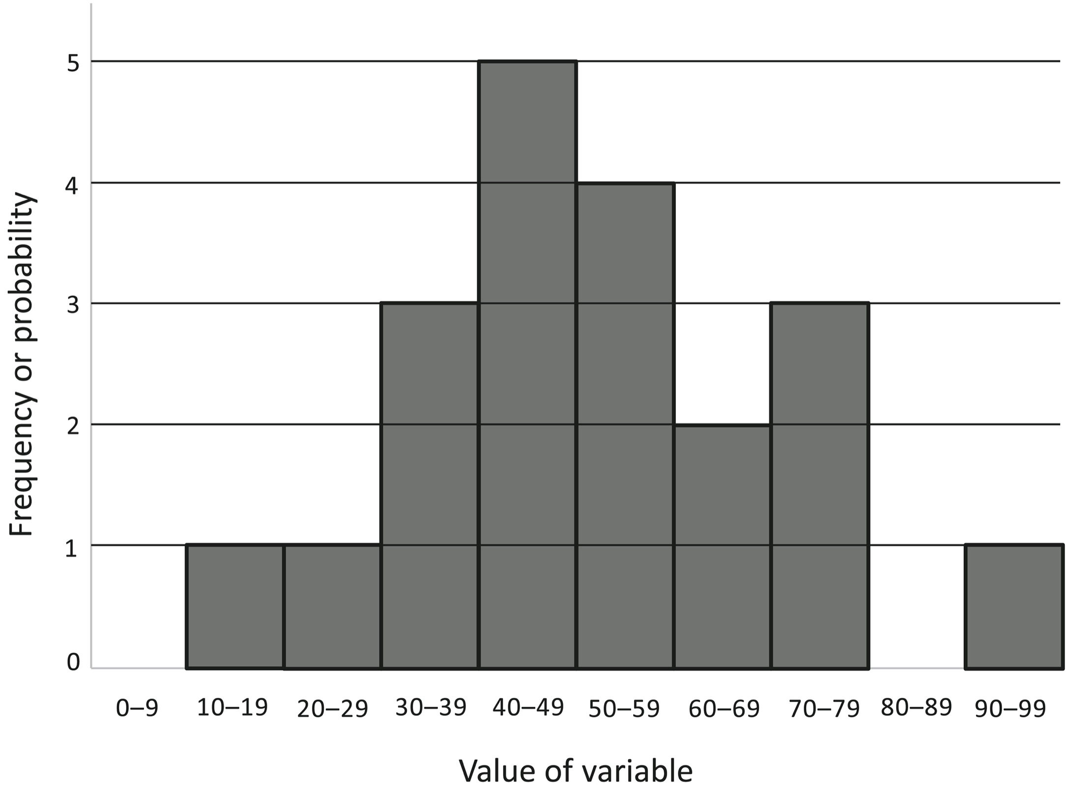
Now imagine that we tested several million people, enough so that we no longer have to sort them into bins but can arrange them left to right by their original scores. As we pile up more and more squares and stand farther and farther back, the ziggurat will blur into a smooth mound, the familiar bell-shaped curve below. It has lots of observations heaped up at an average value in the middle, and fewer and fewer as you look at values that are smaller and smaller to the left or larger and larger to the right. The most familiar mathematical model for a bell curve is called the normal or Gaussian distribution.
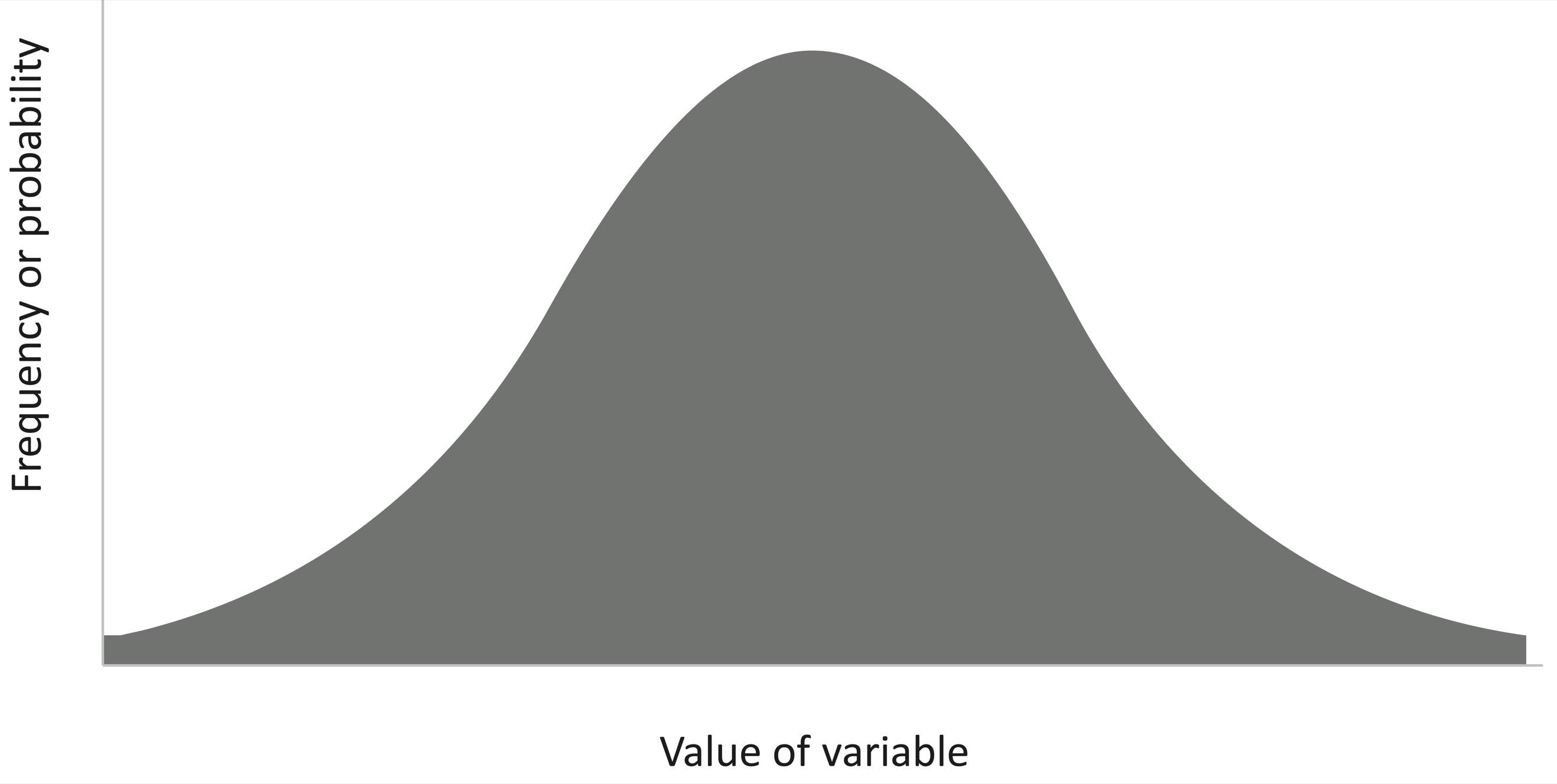
Bell curves are common in the world, such as scores on personality or intelligence tests, heights of men or women, and the speeds of cars on a highway. Bell curves are not the only way that observations can stack up. There are also two-humped or bimodal distributions, such as men’s relative degree of sexual attraction to women and to men, which has a large peak at one end for heterosexuals and a smaller peak at the other end for homosexuals, with still fewer bisexuals in between. And there are fat-tailed distributions, where extreme values are rare but not astronomically rare, such as the populations of cities, the incomes of individuals, or the number of visitors to websites. Many of these distributions, such as those generated by “power laws,” have a high spine on the left with lots of low values and a long, thick tail on the right with a modicum of extreme ones.4 But bell curves—unimodal, symmetrical, thin-tailed—are common in the world; they arise whenever a measurement is the sum of a large number of small causes, like many genes together with many environmental influences.5
Let’s turn to the subject at hand, observations on whether or not something happened in the world. We can’t divine it perfectly—we’re not God—but only through our measurements, such as blips on a radar screen coming from an aircraft, or the opacity of blobs on a scan from a tumor. Our measurements don’t come out precisely the same, on the dot, every time. Instead they tend to be distributed in a bell curve, shown in the diagram below. You can think of it as a plot of the Bayesian likelihood: the probability of an observation given that a signal is present.6 On average the observation has a certain value (the dashed vertical line), but sometimes it’s a bit higher or lower.

But here’s a tragic twist. You might think that when nothing is happening in the world—no bomber, no tumor—we’d get a measurement of zero. Unfortunately, that never happens. Our measurements are always contaminated by noise—radio static, nuisances like flocks of birds, harmless cysts that show up on the scan—and they, too, will vary from measurement to measurement, falling into their own bell curve. More unfortunate still, the upper range of the measurements triggered by noise can overlap with the lower range of the measurements triggered by the thing in the world:
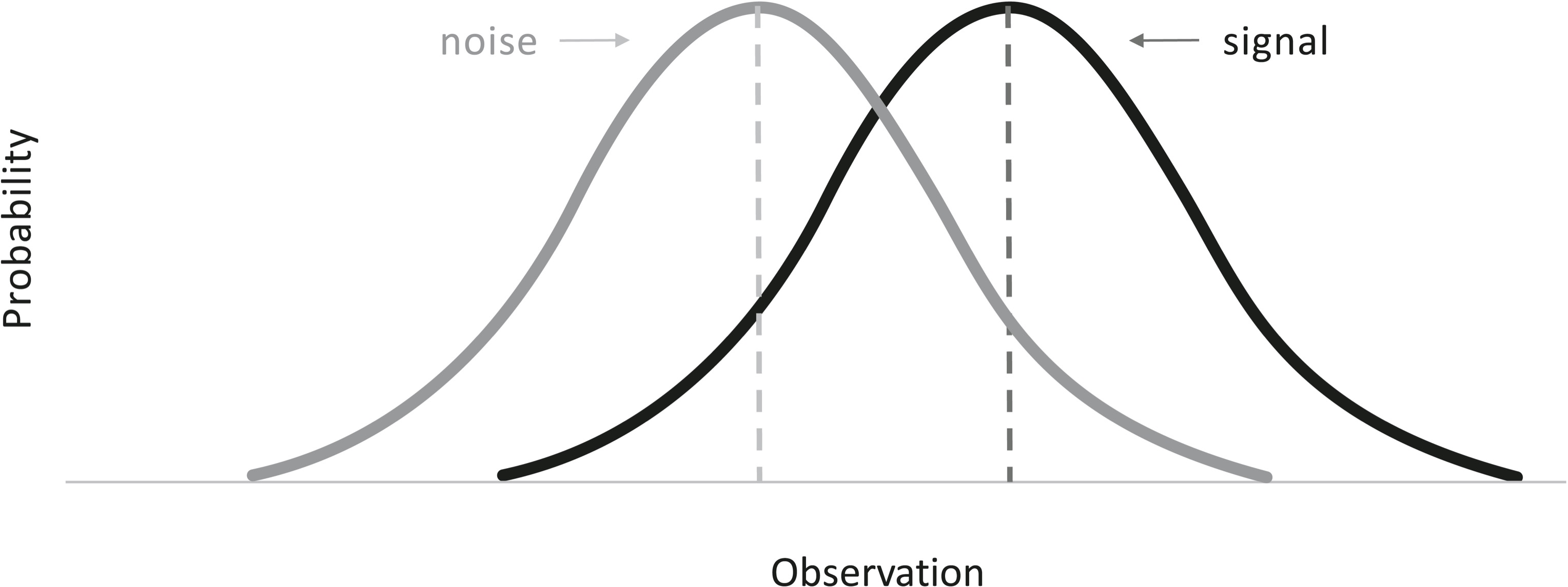
The tragedy is that only God can see the diagram and know whether an observation comes from a signal or from noise. All we mortals see are our observations:

When we are forced to guess whether an observation is a signal (reflecting something real) or noise (the messiness in our observations), we have to apply a cutoff. In the jargon of signal detection, it’s called the criterion or response bias, symbolized as β (beta). If an observation is above the criterion, we say “Yes,” acting as if it is a signal (whether or not it is, which we can’t know); if it is below, we say “No,” acting as if it is noise:

Let’s rise back to the God’s-eye view and see how well we do, on average, with this cutoff. There are four possibilities. When we say “Yes” and it really is a signal (the bomber or tumor is there), it’s called a hit, and the proportion of signals that we correctly identify is shown as the dark shaded portion of the distribution:
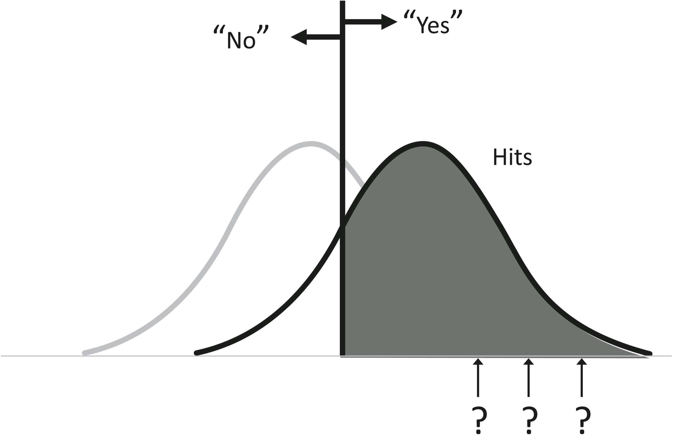
What if it was nothing but noise? When we say “Yes” to nothing, it’s called a false alarm, and the proportion of these nothings in which we jump the gun is shown below as the medium-gray portion:
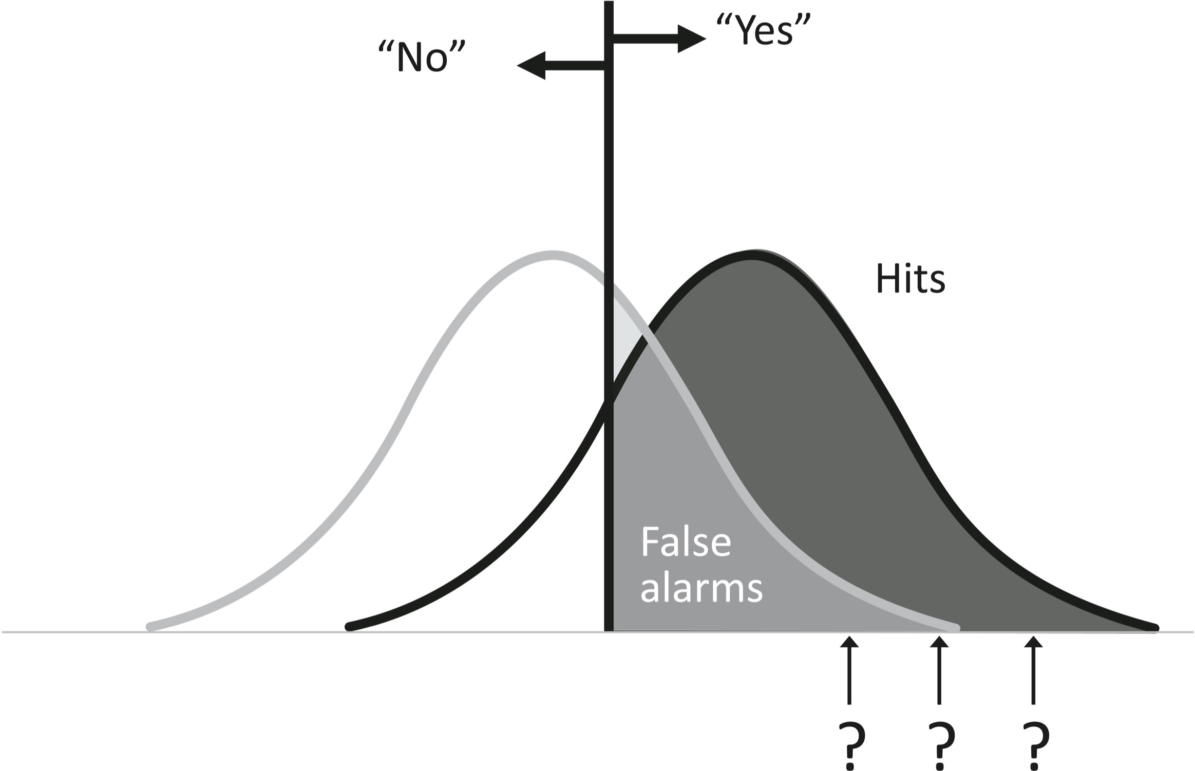
What about the occasions when the observation falls below our criterion and we say “No”? Again, there are two possibilities. When there really is something happening in the world, it’s called a miss. When there is nothing but noise, it’s called a correct rejection.

Here is how the four possibilities carve up the space of happenings:

Since we say “Yes” or “No” every time, the proportions of hits and misses when there is a real signal (right heap) must add up to 100 percent. So must the proportions of false alarms and correct rejections when there’s nothing but noise (left heap). If we were to lower our criterion leftward, becoming more trigger-happy, or raise it rightward, becoming more gun-shy, then we would be trading hits for misses, or false alarms for correct rejections, as a matter of sheer arithmetic. Less obviously, because the two curves overlap, we would also be trading hits for false alarms (when we say “Yes”) and misses for correct rejections (when we say “No”). Let’s have a closer look at what happens when we relax the response criterion, becoming more trigger-happy or yea-saying:
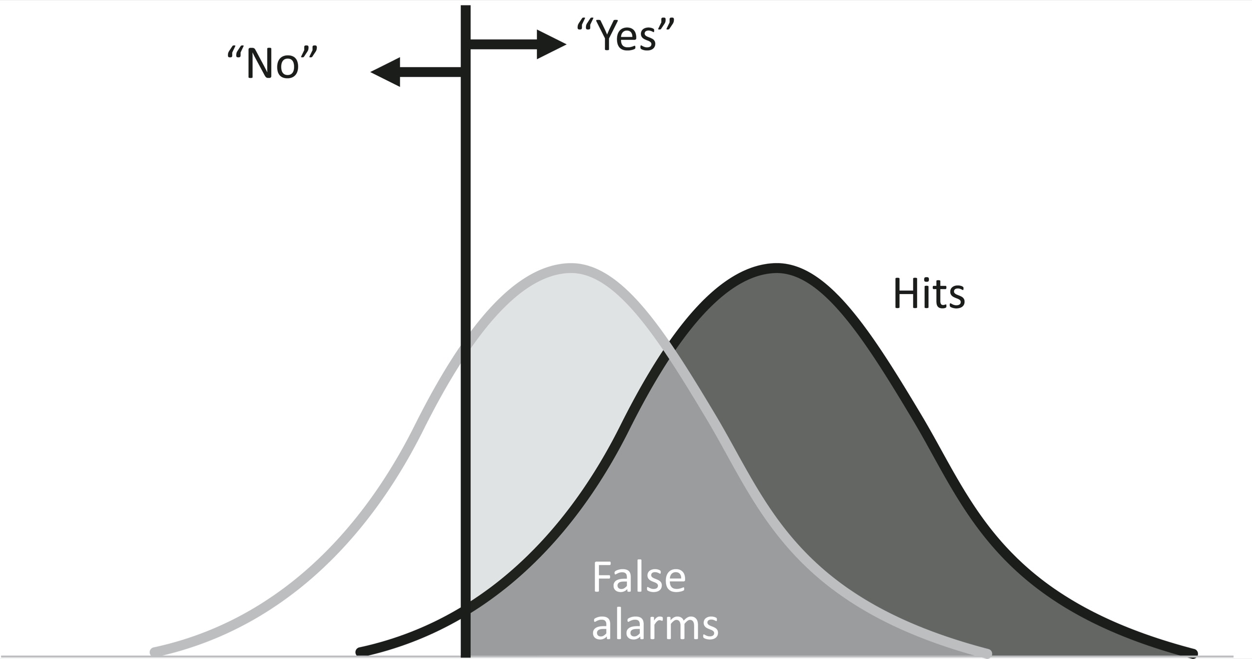
The good news is that we have more hits, catching almost every signal. The bad news is that we have more false alarms, jumping the gun a majority of the time when there’s nothing but noise. What if instead we adopt a more stringent response bias, becoming a gun-shy naysayer who demands a high burden of proof?

Now the news is reversed: we hardly ever cry wolf with a false alarm, which is good, but we miss most of the signals, which is bad. In the extreme case, if we mindlessly said “Yes” every time, we’d always be right when there was a signal and would always be wrong when there was noise, and vice versa if we said “No” every time.
This sounds obvious, but confusing response bias with accuracy by looking only at the signals or only at the noise is a surprisingly common fallacy. Suppose an examiner separately analyzes performance on the true and false items in a true-false test. He thinks he’s seeing whether people are better at detecting truths or rejecting falsehoods, but all he’s really seeing is whether they’re the kind of person who likes saying “Yes” or “No.” I was appalled when a doctor gave me a hearing test that presented a series of beeps increasing in loudness from inaudible to unmissable and asked me to raise a finger when I started hearing them. It wasn’t a test of my hearing. It was a test of my impatience and my willingness to go out on a limb when I couldn’t honestly say whether I was hearing a tone or tinnitus. The theory of signal detection provides a number of ways to do this right, including penalizing respondents for false alarms, forcing them to say “Yes” a certain percentage of the time, asking them for a confidence rating instead of a thumbs-up/thumbs-down, and making the test multiple-choice instead of true-false.
Costs and Benefits, and Setting a Cutoff
With the tragic tradeoff between hits and false alarms (or misses and correct rejections), what’s a rational observer to do? Assuming for the moment that we are stuck with the senses and measuring instruments we have, together with their annoyingly overlapping bell curves, the answer comes right out of expected utility theory (chapter 6): it depends on the benefits of each kind of correct guess and the costs of each kind of error.7
Let’s go back to the scenario in which Signal Detection Theory arose, detecting incoming bombers from radar blips. The four possibilities are arrayed below, each row representing a state of the world, each column a response of our radar operator, with the outcome listed in each cell:
|
“Yes” |
“No” |
|
|
Signal (bomber) |
Hit (city spared) |
Miss (city bombed) |
|
Noise (seagulls) |
False alarm (wasted mission, escalated tensions) |
Correct rejection (all calm) |
In deciding where to set the criterion for responding, our decision maker has to ponder the combined costs (the expected utility) of each column.8 “Yes” responses will spare the targeted city when it truly is under attack (a hit), which is a massive benefit, while incurring a moderate cost when it is not (a false alarm), including the waste of sending interceptor planes scrambling for no reason, together with fear at home and tensions abroad. “No” responses will expose a city to the attack when there is one (a miss), a massive cost, while keeping the blessed peace and quiet when there is not (a correct rejection). Overall the balance sheet would seem to call for a low or relatively trigger-happy response criterion: a few days when interceptors are needlessly sent scrambling would seem a small price to pay for the day when it would spare a city from being bombed.
The calculation would be different if the costs were different. Suppose the response was not sending planes to intercept the bombers but sending nuclear-tipped ICBMs to destroy the enemy’s cities, guaranteeing a thermonuclear World War III. In that case the catastrophic cost of a false alarm would call for being absolutely sure you are being attacked before responding, which means setting the response criterion very, very high.
Also relevant are the base rates of the bombers and seagulls that trigger those blips (the Bayesian priors). If seagulls were common but bombers rare, it would call for a high criterion (not jumping the gun), and vice versa.
As we saw in the previous chapter, we face the same dilemma on a personal scale in deciding whether to have surgery in response to an ambiguous cancer test result:
|
“Yes” |
“No” |
|
|
Signal (cancer) |
Hit (life saved) |
Miss (death) |
|
Noise (benign cyst) |
False alarm (pain, disfigurement, expense) |
Correct rejection (life as usual) |
So where, exactly, should a rational decision maker—an “ideal observer,” in the lingo of the theory—place the criterion? The answer is: at the point that would maximize the observer’s expected utility.9 It’s easy to calculate in the lab, where the experimenter controls the number of trials with a beep (the signal) and no beep (the noise), pays the participant for each hit and correct rejection, and fines her for every miss and false alarm. Then a hypothetical participant who wants to make the most money would set her criterion according to this formula, where the values are the payoffs and penalties:

The exact algebra is less important than simply noticing what’s on the top and the bottom of the ratio and what’s on each side of the minus sign. An ideal observer would set her criterion higher (need better evidence before saying “Yes”) to the degree that noise is likelier than a signal (a low Bayesian prior). It’s common sense: if signals are rare, you should say “Yes” less often. She should also set a higher bar when the payoffs for hits are lower or for correct rejections are higher, while the penalties for false alarms are higher or for misses are lower. Again, it’s common sense: if you’re paying big fines for false alarms, you should be more chary of saying “Yes,” but if you’re getting windfalls for hits, you should be more keen. In laboratory experiments participants gravitate toward the optimum intuitively.
When it comes to decisions involving life and death, pain and disfigurement, or the salvation or destruction of civilization, assigning numbers to the costs is obviously more problematic. Yet the dilemmas are just as agonizing if we don’t assign numbers to them, and pondering each of the four boxes, even with a crude sense of which costs are monstrous and which bearable, can make the decisions more consistent and justifiable.
Sensitivity versus Response Bias
Tradeoffs between misses and false alarms are agonizing, and can instill a tragic vision of the human condition. Are we mortals perpetually doomed to choose between the awful cost of mistaken inaction (a city bombed, a cancer left to spread) and the dreadful cost of mistaken action (a ruinous provocation, disfiguring surgery)? Signal Detection Theory says we are, but it also shows us how to mitigate the tragedy. We can bend the tradeoff by increasing the sensitivity of our observations. The costs in a signal detection task depend on two parameters: where we set the cutoff (our response bias, criterion, trigger-happiness, or β), and how far apart the signal and noise distributions are, called the “sensitivity,” symbolized as dʹ, pronounced “d-prime.”10
Imagine that we perfected our radar so that it weeds out the seagulls, or at worst registers them as faint snow, while displaying the bombers as big bright spots. That means the bell curves for the noise and signal would be pushed farther apart (lower diagram). This in turn means that, regardless of where you put the response cutoff, you will have both fewer misses and fewer false alarms:

And, by the laws of arithmetic, you will enjoy a greater proportion of hits and correct rejections. While sliding the cutoff back and forth tragically trades off one error for another, pulling the two curves apart—better instruments, more sensitive diagnostics, more reliable forensics—is an unmitigated good, reducing errors of both types. Enhancing sensitivity should always be our aspiration in signal detection challenges, and that brings us to one of its most important applications.
Signal Detection in the Courtroom
An investigation into a wrongdoing is a signal detection task. A judge, jury, or disciplinary panel is faced with evidence about the possible malfeasance of a defendant. The evidence varies in strength, and a given body of evidence could have arisen from the defendant having committed the crime (a signal) or from something else, like another person having done the deed or no crime having taken place at all (noise).
The distributions of evidence overlap more than most people appreciate. The advent of DNA fingerprinting (a giant leap in sensitivity) has shown that many innocent people, some on death row, were convicted on the basis of evidence that could have come from noise almost as often as from a signal. The most notorious is eyewitness testimony: research by Elizabeth Loftus and other cognitive psychologists has shown that people routinely and confidently recall seeing things that never happened.11 And most of the sciency-techy-looking methods featured in CSI and other forensic TV shows have never been properly validated but are shilled by self-proclaimed experts with all their overconfidence and confirmation biases. These include analyses of bullets, bite marks, fibers, hair, shoe prints, tire tracks, tool marks, handwriting, blood spatters, fire accelerants, even fingerprints.12 DNA is the most reliable forensic technique, but remember the difference between a propensity and a frequency: some percentage of DNA testimony is corrupted by contaminated samples, botched labels, and other human error.
A jury faced with noisy evidence has to apply a criterion and return a yes-or-no verdict. Its decision matrix has costs and benefits that are reckoned in practical and moral currencies: the malefactors who are removed from the streets or allowed to prey on others, the abstract value of justice meted out or miscarried.
|
“Convict” |
“Acquit” |
|
|
Signal (guilty) |
Hit (justice done; criminal incapacitated) |
Miss (justice denied; criminal free to prey on others) |
|
Noise (innocent) |
False alarm (miscarriage of justice; an innocent punished) |
Correct rejection (justice done; though with costs of a trial) |
As we saw in the discussion of forbidden base rates (chapter 5), no one would tolerate a justice system that worked purely on the practical grounds of the costs and benefits to society; we insist on fairness to the individual. But given that juries lack divine omniscience, how should we trade off the incommensurable injustices of a false conviction and a false acquittal? In the language of signal detection, where do we place the response criterion?
The standard presumption has been to assign a high moral cost to false alarms. As the jurist William Blackstone (1723–1780) put it in his eponymous rule, “It is better that ten guilty persons escape than that one innocent suffer.” And so juries in criminal trials make a “presumption of innocence,” and may convict only if the defendant is “guilty beyond a reasonable doubt” (a high setting for β, the criterion or response bias). They may not convict based on a mere “preponderance of the evidence,” also known as “fifty percent plus a feather.”
Blackstone’s 10:1 ratio is arbitrary, of course, but the lopsidedness is eminently defensible. In a democracy, freedom is the default, and government coercion an onerous exception that must meet a high burden of justification, given the awesome power of the state and its constant temptation to tyrannize. Punishing the innocent, particularly by death, shocks the conscience in a way that failing to punish the guilty does not. A system that does not capriciously target people for ruination marks the difference between a regime of justice and a regime of terror.
As with all settings of a response criterion, the setting based on Blackstone’s ratio depends on the valuation of the four outcomes, which may be contested. In the wake of 9/11, the administration of George W. Bush believed that the catastrophic cost of a major terrorist act justified the use of “enhanced interrogation,” a euphemism for torture, outweighing the moral cost of false confessions by tortured innocents.13 In 2011, the US Department of Education set off a firestorm with a new guideline (since rescinded) that colleges must convict students accused of sexual misconduct based on a preponderance of the evidence.14 Some defenders of such policies acknowledged the tradeoff but argued that sexual infractions are so heinous that the price of convicting a few innocents is worth paying.15
There is no “correct” answer to these questions of moral valuation, but we can use signal detection thinking to ascertain whether our practices are consistent with our values. Suppose we believe that no more than one percent of guilty people should be acquitted and no more than one percent of the innocent convicted. Suppose, too, that juries were ideal observers who applied Signal Detection Theory optimally. How strong would the evidence have to be to meet those targets? To be precise, how large does dʹ have to be, namely the distance between the distributions for the signal (guilty) and the noise (innocent)? The distance may be measured in standard deviations, the most common estimate of variability. (Visually it corresponds to the width of the bell curve, that is, the horizontal distance from the mean to the inflection point, where convex shifts to concave.)
The psychologists Hal Arkes and Barbara Mellers did the math and calculated that to meet these goals the dʹ for the strength of evidence would have to be 4.7—almost five standard deviations separating the evidence for guilty parties from the evidence for innocent ones.16 That’s an Olympian level of sensitivity which is not met even by our most sophisticated medical technologies. If we were willing to relax our standards and convict up to 5 percent of the innocent and acquit 5 percent of the guilty, dʹ would “only” have to be 3.3 standard deviations, which is still a princess-and-the-pea level of sensitivity.
Does this mean that our moral aspirations for justice outstrip our probative powers? Almost certainly. Arkes and Mellers probed a sample of students to see what those aspirations really are. The students ventured that a just society should convict no more than 5 percent of the innocent and acquit no more than 8 percent of the guilty. A sample of judges had similar intuitions. (We can’t tell whether that’s more or less stringent than Blackstone’s ratio because we don’t know what percentage of defendants really are guilty.) These aspirations demand a dʹ of 3.0—the evidence left by guilty defendants would have to be three standard deviations stronger than the evidence left by innocent ones.
How realistic is that? Arkes and Mellers dipped into the literature on the sensitivity of various tests and techniques and found that the answer is: not very. When people are asked to distinguish liars from truth-tellers, their dʹ is approximately 0, which is to say, they can’t. Eyewitness testimony is better than that, but not much better, at a modest 0.8. Mechanical lie detectors, that is, polygraph tests, are better still, around 1.5, but they are inadmissible in most courtrooms.17 Turning from forensics to other kinds of tests to calibrate our expectations, they found dʹs of around 0.7 for military personnel screening tests, 0.8–1.7 for weather forecasting, 1.3 for mammograms, and 2.4–2.9 for CT scans of brain lesions (estimated, admittedly, for the technologies of the late twentieth century; all should be higher today).
Suppose that the typical quality of evidence in a jury trial has a dʹ of 1.0 (that is, one standard deviation higher for guilty than for innocent defendants). If juries adopt a tough response criterion, anchored, say, by a prior belief that a third of defendants are guilty, they will acquit 58 percent of guilty defendants and convict 12 percent of the innocent ones. If they adopt a lax one, corresponding to a prior belief that two thirds of defendants are guilty, they’ll acquit 12 percent of guilty defendants and convict 58 percent of innocent ones. The heart-sinking conclusion is that juries acquit far more guilty people, and convict far more innocent ones, than any of us would deem acceptable.
Now, the criminal justice system may strike a better bargain with the devil than that. Most cases don’t go to trial but are dismissed because the evidence is so weak, or plea-bargained (ideally) because the evidence is so strong. Still, the signal detection mindset could steer our debates on judicial proceedings toward greater justice. Currently many of the campaigns are naïve to the tradeoff between hits and false alarms and treat the possibility of false convictions as inconceivable, as if the triers of fact were infallible. Many advocates of justice, that is, argue for pulling the decision cutoff downward. Put more criminals behind bars. Believe the woman. Monitor the terrorists and lock them up before they attack. If someone takes a life, they deserve to lose their own. But of mathematical necessity, lowering the response criterion can only trade one kind of injustice for another. The arguments could be restated as: Put more innocent people behind bars. Accuse more blameless men of rape. Lock up harmless youths who shoot off their mouths on social media. Execute more of the guiltless.18 These paraphrases do not, by themselves, refute the arguments. At a given time a system may indeed be privileging the accused over their possible victims or vice versa and be due for an adjustment. And if less-than-omniscient humans are to have a system of justice at all, they must face up to the grim necessity that some innocents will be punished.
But being mindful of the tragic tradeoffs in distinguishing signals from noise can bring greater justice. It forces us to face the enormity of harsh punishments like the death penalty and long sentences, which are not only cruel to the guilty but inevitably will be visited upon the innocent. And it tells us that the real quest for justice should consist of increasing the sensitivity of the system, not its bias: to seek more accurate forensics, fairer protocols for interrogation and testimony, restraints on prosecutorial zealotry, and other safeguards against miscarriages of both kinds.
Signal Detection and Statistical Significance
The tradeoff between hits and false alarms is inherent to any decision that is based on imperfect evidence, which means that it hangs over every human judgment. I’ll mention one more: decisions about whether an empirical finding should license a conclusion about the truth of a hypothesis. In this arena, Signal Detection Theory appears in the guise of statistical decision theory.19
Most scientifically informed people have heard of “statistical significance,” since it’s often reported in news stories on discoveries in medicine, epidemiology, and social science. It’s based on pretty much the same mathematics as Signal Detection Theory, pioneered by the statisticians Jerzy Neyman (1894–1981) and Egon Pearson (1895–1980). Seeing the connection will help you avoid a blunder that even a majority of scientists routinely commit. Every statistics student is warned that “statistical significance” is a technical concept that should not be confused with “significance” in the vernacular sense of noteworthy or consequential. But most are misinformed about what it does mean.
Suppose a scientist observes some things in the world and converts her measurements into data that represent the effect she is interested in, like the difference in symptoms between the group that got the drug and the group that got the placebo, or the difference in verbal skills between boys and girls, or the improvement in test scores after students enrolled in an enrichment program. If the number is zero, it means there’s no effect; greater than zero, a possible eureka. But human guinea pigs being what they are, the data are noisy, and an average score above zero may mean that there is a real difference in the world, or it could be sampling error, the luck of the draw. Let’s go back to the God’s-eye view and plot the distribution of scores that the scientist would obtain if there’s no difference in reality, called the null hypothesis, and the distribution of scores she would obtain if something is happening, an effect of a given size. The distributions overlap—that’s what makes science hard. The diagram should look familiar:

The null hypothesis is the noise; the alternative hypothesis is the signal. The size of the effect is like the sensitivity, and it determines how easy it is to tell signal from noise. The scientist needs to apply some criterion or response bias before breaking out the champagne, called the critical value: below the critical value, she fails to reject the null hypothesis and drowns her sorrows; above the critical value, she rejects it and celebrates—she declares the effect to be “statistically significant.”
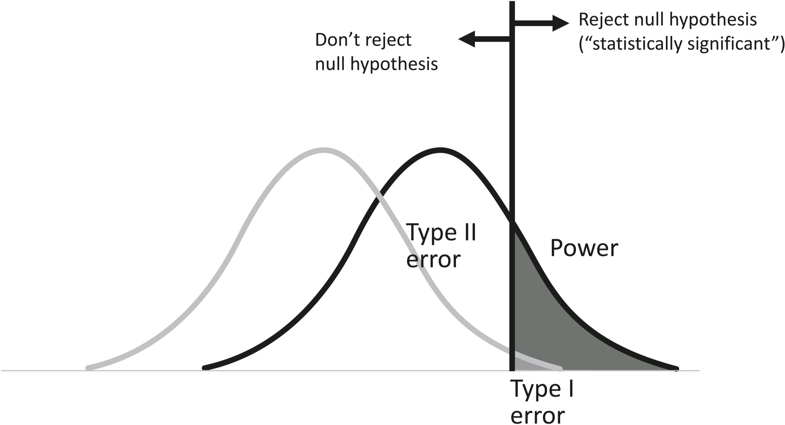
But where should the critical value be placed? The scientist must trade off two kinds of error. She could reject the null hypothesis when it is true, namely a false alarm, or in the argot of statistical decision theory, a Type I error. Or she could fail to reject the null hypothesis when it is false—a miss, or in the patois, a Type II error. Both are bad: a Type I error introduces falsehood into the scientific record; a Type II error represents a waste of effort and money. It happens when the methodology was not designed with sufficient “power” (the hit rate, or 1 minus the Type II error rate) to detect the effect.
Now, deep in the mists of time it was decided—it’s not completely clear by whom—that a Type I error (proclaiming an effect when there is none) is especially damaging to the scientific enterprise, which can tolerate only a certain number of them: 5 percent of the studies in which the null hypothesis is true, to be exact. And so the convention arose that scientists should adopt a critical level that ensures that the probability of rejecting the null hypothesis when it is true is less than 5 percent: the coveted “p < .05.” (Though one might have thought that the costs of a Type II error should also be factored in, as it is in Signal Detection Theory, for some equally obscure historical reason it never was.)
That’s what “statistical significance” means: it’s a way to keep the proportion of false claims of discoveries beneath an arbitrary cap. So if you have obtained a statistically significant result at p < .05, that means you can conclude the following, right?
-
The probability that the null hypothesis is true is less than .05.
-
The probability that there is an effect is greater than .95.
-
If you rejected the null hypothesis, there is less than a .05 chance that you made the wrong decision.
-
If you replicated the study, the chance that you would succeed is greater than .95.
Ninety percent of psychology professors, including 80 percent of those who teach statistics, think so.20 But they’re wrong, wrong, wrong, and wrong. If you’ve followed the discussion in this chapter and in chapter 5, you can see why. “Statistical significance” is a Bayesian likelihood: the probability of obtaining the data given the hypothesis (in this case, the null hypothesis).21 But each of those statements is a Bayesian posterior: the probability of the hypothesis given the data. That’s ultimately what we want—it’s the whole point of doing a study—but it’s not what a significance test delivers. If you remember why Irwin does not have liver disease, why private homes are not necessarily dangerous, and why the pope is not a space alien, you know that these two conditional probabilities must not be switched around. The scientist cannot use a significance test to assess whether the null hypothesis is true or false unless she also considers the prior—her best guess of the probability that the null hypothesis is true before doing the experiment. And in the mathematics of null hypothesis significance testing, a Bayesian prior is nowhere to be found.
Most social scientists are so steeped in the ritual of significance testing, starting so early in their careers, that they have forgotten its actual logic. This was brought home to me when I collaborated with a theoretical linguist, Jane Grimshaw, who tutored herself in statistics and said to me, “Let me get this straight. The only thing these tests show is that when some effect doesn’t exist, one of every twenty scientists looking for it will falsely claim it does. What makes you so sure it isn’t you?” The honest answer is: Nothing. Her skepticism anticipated yet another explanation for the replicability imbroglio. Suppose that, like Lewis Carroll’s snark hunters, twenty scientists go chasing after a figment. Nineteen file their null results in a drawer, and the one who is lucky (or unlucky) enough to make the Type I error publishes his “finding.”22 In an XKCD cartoon, a pair of scientists test for a correlation between jelly beans and acne separately for each of twenty colors, and become famous for linking green jellybeans to acne at p < .05.23 Scientists have finally gotten the joke, are getting into the habit of publishing null results, and have developed techniques to compensate for the file drawer problem when reviewing the literature in a meta-analysis, a study of studies. Null results are conspicuous by their absence, and the analyst can detect the nothing that is not there as well as the nothing that is.24
The scandalous misunderstanding of significance testing bespeaks a human yearning. Philosophers since Hume have noted that induction—drawing a generalization from observations—is an inherently uncertain kind of inference.25 An infinite number of curves can be drawn through any finite set of points; an unlimited number of theories are logically consistent with any body of data. The tools of rationality explained in these chapters offer different ways of coping with this cosmic misfortune. Statistical decision theory cannot ascertain the truth, but it can cap the damage from the two kinds of error. Bayesian reasoning can adjust our credence in the truth, but it must begin with a prior, with all the subjective judgment that goes into it. Neither one provides what everyone longs for: a turnkey algorithm for determining the truth.