Figure 5.1. The variation in EVCRACK.1
5
MEASUREMENT
Having walked through the Wheel of Science and given an overview of the process of science, we now turn to addressing some of the building blocks that help us move between theory and hypotheses to observation. Once our theories are formalized into testable hypotheses, we need to take a closer look at the variables including expanding on what variables are (versus constants), what we mean by “variance,” and how to operationalize variables and to recognize levels of measurement.
The primary task of social science is to explain the connection between concepts. We’ve explained that theory allows us to link concepts and that this theoretical pairing is formalized into hypotheses that state relationships between the concepts—how one concept impacts another concept (e.g., we expect that higher levels of education lead to higher levels of income). In order to test our hypotheses, we need to operationalize our concepts—finding indicators that measure concepts. Let’s revisit the relationship between education and income.
Operationalizing concepts simply means that we find variables (measures) of the concepts. If we are interested in operationalizing education and income, we could turn to a national survey (like we did in Chapter 1) and look for variables that measure “education” like “What is the highest level of education you have completed?” and “What was your total family income before taxes last year?” to measure “income.” These two specific measures of education and income are operationalizations: variables that measure the concepts education and/or income.
In Chapter 2 you operationalized variables for the concepts of religiosity, health, and prejudice. When operationalizing a variable two parts are necessary. Variables need to have some sort of descriptor telling us what the variable is measuring, as well as having certain attributes or answer categories. For example, when operationalizing education in our example, the question itself is the descriptor for what is being measured: “What is the highest level of education you have completed?” Since operationalization is a broader process than our focus on survey research items, another example would include our illustration from Chapter 2 of going to a graveyard to operationalize socioeconomic status and health. For this example a descriptor would be the gravestone itself (for both socioeconomic status and age/lifespan).
The second important part of a variable is the attributes or categories. The attributes or categories tell us how the variable is being measured—the descriptor tells us what is being measured, and the categories tell us how the variable is being measured. In the case of the variable we operationalized to measure education, “What is the highest level of education you have completed?” appropriate categories may include “Less than a high school education, a high school education, some college education, a college degree.” We call these “discrete” categories because they are “closed-ended” variables—supplying respondents with a specific, discrete set of responses (we look at these types of variables more closely in Chapter 14 when discussing survey research). For variables that have a limited, or smaller, number of categories, we refer to them as categorical variables or variables that have these discrete, limited number of category options.
For the example measuring socioeconomic status and health in a graveyard, the gravestones used to measure socioeconomic status could have the attributes of small stone, medium stone, or large stone—in effect measuring the size of the stone to denote status (bigger stones indicating higher socioeconomic status, smaller stones lower status). In terms of measuring age, the dates of birth and death would denote age (ages being the attributes) to measure level of health. For any given gravestone, the age will vary into distinct age categories (e.g., 88 years old, 76 years old, 93 years old, 67 years old, 49 years old, etc.). Because each age represents its own category, possible categories range from age = 0 to age = 101 (for example). This age range could then be more than 100 categories. When variables have a broad range of categories (more than 20, for example) we refer to them as continuous variables.
Apart from having attributes that are categorical or continuous, variable categories must also be exhaustive and mutually exclusive. Exhaustive attributes mean that all possible categories are included in the variable. You have probably taken a survey where you know your answer almost before you get to the answer categories. Yet sometimes you find that your answer is not included. What do you do? Do you pick the next best answer or do you skip the question? Do you get frustrated because your answer is not there and stop filling out the survey altogether? Making sure that each variable has exhaustive categories is important. In religion research, it is not uncommon to see a question asking for someone’s religious preference. Look at the following variable:
What is your religious preference?
Given a particular cultural context, these categories may make sense. For example, in the United States, these are the largest religious groups. You probably recognize, however, that the categories are not exhaustive—not everyone fits into these categories. A first reaction might include thinking of all possible religious groups:
What is your religious preference?
We hope you recognize that there are so many varieties of religious preferences that we can never come up with a comprehensive list of all possible religious preferences in order to make the categories exhaustive. There is an easier way to make a question exhaustive:
What is your religious preference?
By adding the categories of “None” and “Other,” the question is now exhaustive. Anyone who does not fit into Protestant, Catholic, or Jewish is some other religious preference or has no religious preference; thus the categories now encompass anyone and everyone.
As well as having exhaustive categories, variables also must have categories that are mutually exclusive. Having mutually exclusive categories means that while everyone can answer one category (Protestant, Catholic, Jewish, None, Other), people should be able to choose only one category. Several years ago a survey associated with a medical school asked respondents the following question:
What is your religious preference?
First of all, without a category for “None,” the question attributes are not exhaustive. The category for “Christian,” however, is problematic because Catholicism is one of two branches of Christianity—they are the same thing. Protestant Christians have only one option here (“Christian”), but what does a Catholic Christian choose? These attributes are not mutually exclusive: Catholics fit into two categories. When attributes are not mutually exclusive, respondents are misclassified; that is, the categories do not reflect the respondent’s true response/classification.
Some questions are designed specifically to have respondents select “all that apply.” We call these “cafeteria” questions, and expect that each category represents a distinctive answer, for which there are multiple categories. When you have a question that is expected to be one answer per respondent, variable attributes should be both exhaustive (everyone can answer at least one) and mutually exclusive (everyone can answer only one).
We are concerned with what variables measure and how variables are measured. When variables have exhaustive and mutually exclusive attributes, they should vary appropriately. We want variables to vary because it is through their variation that we can measure change in another variable. Variation is the amount of change included in a variable; each variable has 100 percent variation.
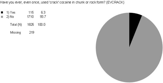
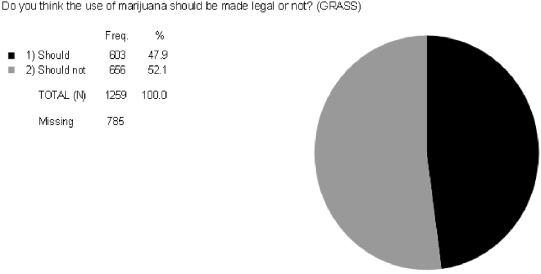
Let’s look at the variance—distribution—of the following two GSS variables. The variable EVCRACK in Figure 5.1 measures whether or not respondents have ever used crack cocaine (with answer categories of “yes” or “no”). The variable GRASS in Figure 5.2 measures whether respondents think that marijuana should be made legal (with answer categories of “should” [be made legal] or “should not” [be made legal]).
Figure 5.1. The variation in EVCRACK.1
Figure 5.2. The variation in GRASS.1
Both of the variables in Figures 5.1 and 5.2 are considered dichotomous variables because they each have two category options (yes/no and should/should not, respectively). Think about each of these variables as having 100 percent variation. In each of these examples, variation is split into two attributes. For EVCRACK, 6.3 percent of people report having ever tried crack cocaine; 93.7 percent of people report not having tried crack cocaine. The closer a variable gets to having any one category reach 100 percent, the less variance there is in the variable. When most people select the same response, a variable has little variance.
In contrast, the variable GRASS has a nearly maximum amount of variation. Those responding that marijuana should be made legal versus should not be made legal are 47.9 percent to 52.1 percent, respectively. For a dichotomous variable (a variable with two answer categories), the maximum amount of variation is 50 percent for each category. Unlike EVCRACK, GRASS has almost as much variation as possible.
Here are two additional dichotomous variables. Look at Figure 5.3 for the variation in the variable for POSTLIFE, which measures whether or not a person believes there is a life after death, and Figure 5.4 for the variation in ASTROLGY, which measures whether respondents ever read a horoscope or their personal astrology report.
Figure 5.3. The variation in POSTLIFE.1
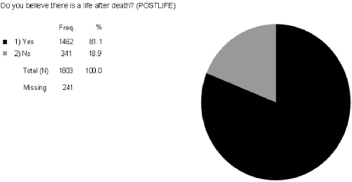
Figure 5.4. The variation in ASTROLGY.1
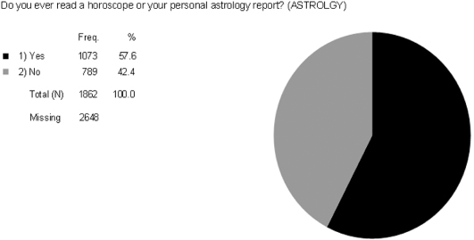
Which of these two variables has the most variation? Figure 5.3 shows the univariate distribution for POSTLIFE with 81.1 percent of people reporting that they believe in a life after death while 18.9 percent of people report they do not believe in a life after death. The results in Figure 5.4 for ASTROLGY show that 57.6 percent of respondents read a horoscope or a personal astrology report, and 42.4 percent of respondents do not. Remember that the maximum variation for a dichotomous variable is for each of the two categories to be closer to 50 percent. That makes ASTROLGY the variable with the most variation (as opposed to POSTLIFE).
When using a dichotomous variable (a variable with only two attributes/answer categories), variation is important to gauge. A widely used rule for dichotomous variables is that they need to have at least 20 percent or more variation between categories. If one category encompasses less than 20 percent of the respondents, there’s often not enough variation within the variable to use it to explain the change/variation in another variable. The more variance within a variable, the better able that variable is to explain variance in another variable.
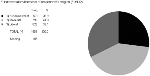
One way to increase variation in a variable is to increase the number of answer categories. By adding a third answer category to the variable FUND 2 in Figure 5.5, we have created more variation. What would maximum variation be for FUND2, which measures the fundamentalism/liberalism of respondent’s religion? If each variable contains 100 percent variance, to attain maximum variance a variable with three categories would have categories that approach 33 percent (100 percent variation/3 categories). FUND2 is fairly evenly distributed between categories.
Figure 5.5. The variation in FUND2.1
What about the distribution of POLVIEWS? With seven category answers, we have a lot of variation. Notice the largest part of the pie chart has “Moderates” representing 37.8 percent of the variance. With more categories of somewhat even distribution between options for “liberal” and “conservative,” there seems to be ample variation. Of course, we can collapse the POLVIEWS variable to get a better sense of how the distribution works by including all three categories that measure conservative and liberal.
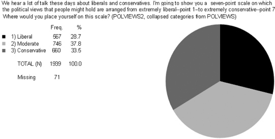
The POLVIEWS2 variable shown in Figure 5.7 has slightly more variation than the FUND2 variable in Figure 5.6, since each category of POLVIEWS2 is closer to the 33 percent of maximum variation expected in a variable with three categories. Social researchers are interested in variation because higher variation in one variable helps to explain variation in other variables. Sometimes, however, variables that appear to have variation have no variation at all; these are called constants.
Figure 5.6. The variation in POLVIEWS.1
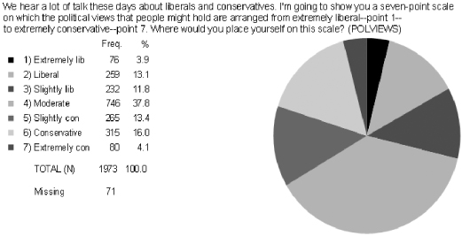
Figure 5.7. The variation within POLVIEWS2.1
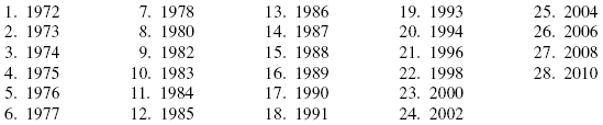
When looking at the variance of a variable, you want to make sure that you do not accidentally confuse a constant for a variable. A constant has a value that does not change—it has no variation. The GSS has been conducted most years since 1972, and then biennially beginning in 1994. One of the items contained in each GSS is the variable YEAR, or “GSS year for this respondent.” Since the GSS uses multiple survey years to conduct time-trend studies, it is important to have a variable that allows us to control for year of survey given. When a codebook is created, each year that the survey has been conducted is included as an answer category, so the descriptor and attributes might appear in the codebook with a list of attributes for each GSS year like this:
GSS Year for the Respondent
The number of categories for the variable indicates that the variable has a good amount of variation. Yet when you run a univariate statistic on the variable for the GSS 2010, 100 percent of the respondents give the same answer, shown in Figure 5.8.
Figure 5.8. The variation in YEAR for GSS 2010.
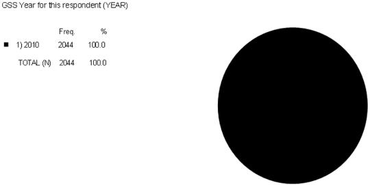
While YEAR may appear to be a variable because the categories are coded for each possible year the GSS has been administered, the actual value for a given year will not change because all of the respondents will have the same value (same year). YEAR is therefore a constant and not a variable when used in the GSS 2010. When looking at more complex variables, you need to make sure enough variation (change) exists within one variable to explain the change within another variable.
Levels of measurement help us think about what variables tell us. Depending on how a variable is measured, we can also tell what statistical analysis is best for the type of information contained in a variable. For example, we’ve been using cross-tabulation analysis to look at research questions. The variables that are most appropriate to cross-tabular analysis are those that have seven or fewer categories—the categorical variables we discussed in a previous section. Categorical variables tend to be nominal- or ordinal-level variables, but they can be created from any level of data. For example, we noted earlier that in eliciting variation for a variable, it is better to get the most variation. Most surveys ask respondents about their age. It is much better to begin with a question such as, “What is your age? ____________,” or “In what year were you born?” to allow respondents to give you their actual age. Asking their exact age or year of birth gives us the maximum variation. Once you have an actual age (which is a ratio-level variable), you can create a categorical variable that groups the age variable into smaller categories (e.g., “younger than 18 years old, 18 to 29 years old, 30 to 39 years old, 40 to 49 years old, 50 to 59 years old, 60 to 69 years old, 70 years old or older). This categorical variable is now an ordinal-level variable.
There are four levels of measurement: nominal, ordinal, interval, and ratio. Each subsequent level of measurement builds on the previous level, adding a unique quality for that level (while each of the four levels of measurement distinctly describe what is being measured by a variable, as we move from nominal to ordinal to interval to ratio, each next level takes on an additional quality, like having an inherent order). The first level of measurement is the nominal level. The categories/attributes for a nominal-level variable distinctly describe that variable. For example, look at the variable REG16:
In what state or foreign country were you living when you were 16?
A nominal measure distinctively describes the variable by the answer categories/attributes of the variable (as we mentioned before, the descriptor tells you what the variable measures—“In what state or foreign country were you living when you were 16?”—while the categories tell you how the variable is measured). Does each category of REG16 give you a clear, distinctive description of which category of the country you lived in at 16? Each of the answer categories distinctly describes in what region of the county a respondent lived at 16. There is no inherent order to the list of attributes (at least from a scientific perspective—our students generally try to explain why the Pacific region is better than the others); each attribute simply describes a region of the country. None is higher, bigger, or faster than the other. Each is simply distinct.
Ordinal measures are the next level of measurement. Like nominal measures, ordinal measures have answer categories that distinctively describe the variable. Ordinal measures, however, can also be ordered along some kind of continuum, allowing us to rank them logically. Look at the variable for SOCBAR.
How often do you do the following things: Go to a bar or tavern?
Notice that the categories have a logical order that tell us how more or less frequently respondents spend time in a bar or tavern. Ordinal measures are useful because we can compare respondents’ frequency of going to a bar, making clearer generalizations, like “the more often one goes to a bar or tavern, the less likely they are to attend church.”
Frequency of religious attendance would be another example of an ordinal measure:
How often do you attend religious services?
As long as the categorical attributes of a variable can be ordered along some sort of a continuum, the minimum level of measurement would be ordinal.
The next level of measurement is the interval level. Interval measures build on the previous two levels; interval measures have answer categories that distinctly describe the variable like nominal and ordinal measures, and they can also be ranked logically in some kind of order like ordinal measures. The unique quality that interval-level measures add to data is that interval measures also have equal distance between units. Whereas an ordinal-level variable ranks the categories within groupings, interval-level measures give a more precise degree of difference between categories by telling us how much more one category is than another.
For example, if I asked, “What is the current temperature?” Depending on where you live and what season it is, you could give answers like, “72 degrees” or “37 degrees.” The temperature would be a good example of an interval-level variable, where the assumption is that each degree is an equal measure of temperature. So the difference between 72 and 37 degrees is 35 degrees, just as the difference between 10 and 45 is 35 degrees. We can say that because we know that each degree measures the same unit—degrees. Interval measures are generally considered continuous variables because they are structured in such a way as to maximize variation (creating many attributes).
Interval measures, however, are made somewhat more unique because they contain no meaningful zero point. What is a meaningful zero point? We expect that when a variable is measured at “zero” that zero is the absence of the variable altogether. So when you answer “zero” to a question like, “How many classes did you skip last semester?” we expect that no classes—zero classes—were skipped last semester. Interval-level measures, however, are unique. When we say it’s zero degrees outside, that does not mean there is no more temperature. Temperatures are measured below zero, into the negatives. Thus temperature has no meaningful zero point. This makes interval measures somewhat unique.
Using the same building blocks within levels of measurement—distinctively describing a variable, being logically ordered along some continuum, and having equal distance between units—are ratio measures. Ratio-level measures expand interval-level measures by having a meaningful zero point—at the measure of zero, there is no more of the variable. Because ratio measures have a meaningful zero point, we can talk about ratios (2 times, half as much, fourfold.). For example, if Ernie weighs 220 pounds and Bert weighs 110 pounds, we can say that Ernie weighs twice as much as Bert. Weight would be an example of a ratio measure.
Another example of a ratio measure would be:
How many children do you have?
In this variable, each category represents the actual number of children a person has (equal distance between units); therefore, the variable is a ratio measure. Having “zero” children means that the respondent has no children.
We can take the same concept—even the same variable—and measure it using multiple levels of measurement depending on what we want to learn about the variables or glean from a particular analysis. As we’ve explained, if variables initially elicit the maximum variation, different analyses can be used based on the interval- or ratio-level measure while the measure can be collapsed as an ordinal or nominal measure to use in cross-tabular analyses. For example, the variable that measures “Number of hours worked last week” can be measured in two ways. The first variable describes “Number of hours worked last week” and is asked as an open-ended question (one where respondents fill in their own answers), eliciting the maximum variation (with a range of working 0 to 168 hours per week)2. What level of measurement is this? Does each hour given describe how many hours the respondent worked? Yes, so minimally the variable is nominal. Are the categories ordered on any kind of a continuum? Yes, lower categories indicate fewer working hours and vice versa, which would mean we’ve moved to the ordinal level. Does each category have equal distance between units? Yes, each category represents an hour; for one respondent who worked 40 hours, he or she would have worked 20 hours less than someone who worked 60 hours or 128 hours less than someone who worked 24 hours a day, 7 days a week. Therefore we’ve moved up to the interval level of measurement. Last question: do the categories have a meaningful zero point? In other words, do those who report working zero hours last week mean that they did no work at all? Yes. Thus the categories for this variable are ratio-level measures.
Of course, if we want to do a cross-tabular analysis, having 169 possible categories is daunting (168 possible hours per week plus the category of zero hours is 169 total category possibilities). How would you be able to represent or read this data in a 2 × 2 cross-tab? In order to do a cross-tabular analysis, we need a categorical variable. Taking the original variable, we can collapse the categories into meaningful groups that denote those who work less than full time, full time, and more than full time. We do this by combining all the hours between 0 and 39 to represent less than full time, keep 40 hours as the category for full time, and take categories 41 to 168 as working more than full time. These then become “less than 40 hours,” “40 hours,” and “more than 40 hours” worked last week. What level of measurement do we now have? Does each category describe how many hours the respondent worked? Yes, so minimally the variable is nominal. Are the categories ordered on any kind of a continuum? Yes, lower categories indicate fewer working hours and vice versa, which would mean we’ve moved to the ordinal level. Does each category have equal distance between units? No. Of the three categories, 1, 2, and 3, each is composed of unequal units; that is, the category for working less than 40 hours has at least 40 possible hours in it; the category for worked 40 hours has only one hour, the category for 40 to 168 hours worked has many more. The categories—1, 2, and 3—are not measured using the same units. Therefore the variable does not meet the criteria for an interval measure and must then be an ordinal measure.
Now that we’ve looked at how variables are measured, we address units of analysis, the things a hypothesis directs us to observe, or the cases in a data set (the thing being studied). Two general categories of units include individual-level units (people) and aggregate-level units (geographic places—states, nations or things—and social units— churches, schools, clubs, etc.). Aggregate units are single units (like states) that are composed of individuals. Units of analysis are the things that have the variables. Let’s go back to the relationship between education and income. If we hypothesize that higher levels of education lead to higher levels of income, we want to identify the independent and dependent variables. Independent variables are our starting point. We assume (infer) that the independent variable is causing changes to a second variable, the dependent variable. Our hypothesis implies that if we know a person’s level of education, we can predict that person’s level of income. So education is the independent variable (the causal variable) and income is the dependent variable (the effect).
To understand units of analysis, you want to ask the question, “Who or what can have an education level and an income level?” The only thing that can get an education and have income are people/individuals; thus people are the units of analysis. What if our hypothesis stated that countries with a high percentage of the population with college degrees will have a lower percentage of hate crimes? In this hypothesis, who or what has a percentage of the population with college degrees and a percentage of hate crimes? Countries.
When we engage in research, we trust that the measures we use to define a variable actually capture the meaning of the concept and that they do so consistently. These are the considerations of validity in the former instance and reliability in the latter. For purposes of our discussion, we can use the following standard definitions of the concepts:
A research measure can be reliable, but not necessarily valid, as, for example, using height as a measure of athletic prowess. Height can be measured very accurately, but it does not necessarily indicate how much of an athlete a short or tall person may be.
However, a measure may be valid, but it may not have strong reliability as is the case in some glucometers. When people with diabetes check their blood sample for sugar content, they will have a valid measure of blood glucose, but the instrument may give varying readings from day to day (and therefore not a reliable measure) due to a variety of factors (e.g., quality of test strips, etc.).
Notes
1 Pie chart derived using MicroCase Statistical Software.
2 It is not uncommon for some respondents to write in “168” when asked how many hours per week they work. This response indicates that they believe they work 24 hours a day, 7 days a week.