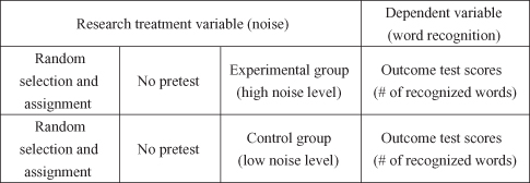
Figure 15.1 The experimental research design specification: t test with two groups.
15
STATISTICAL METHODS OF DIFFERENCE: T TEST1
There are many types of statistical procedures that attempt to detect statistical differences between and among research conditions. We have already looked at chi square, which examines whether the frequencies of the categories of one variable are distributed equally across the categories of another variable. Statistical procedures that use a higher level of data, namely interval data, also detect differences among variables.
Independent t tests determine whether the two categories of a predictor (independent) variable result in statistically different mean values of an outcome (dependent) variable. Thus, do men and women postal workers (independent variable) indicate different levels of job satisfaction (dependent variable)? This procedure assumes that the predictor categories are “independent,” or unrelated to one another. Other t tests can accommodate for the two predictor categories being related or dependent (e.g., when the same people are tested twice as in a pre-post test), but they use different formulas.
ANOVA (analysis of variance) tests do essentially the same thing, but instead of comparing two categories of a predictor variable (or factor), they compare three or more categories. Thus, which of three different instructional methods leads to greater math achievement scores? The added complexity is that the procedure uses special drill-down methods to determine the differences among each of the pairs of categories if the overall test is significant. Thus, if the overall test is significant, are there significant differences between method A and method B, between method A and method C, or between method B and method C? As you can see, the procedure is specific, and the results can get quite involved depending on how many categories there are to compare. Like the “dependent” t test, there are also ANOVA procedures that use related categories and must therefore use special formulas to accommodate for the dependencies (as in within-subjects ANOVA).
We need to be careful to point out, however, that when these procedures are used (in experimental or post facto designs), the researcher needs to ensure that the groups they choose to compare are independent of one another. Independent samples mean that choosing subjects for one group has nothing to do with choosing subjects for the other groups. Thus in experimental situations that involve two groups, if we randomly select Bob and assign him randomly to group 1 (experimental group), it has nothing to do with the fact that we choose Sally and assign her randomly to group 2 (control group). In post facto procedures with two groups, if we compare the job satisfaction of “workers with more than five years on the job” to “workers with five or fewer years on the job,” it is important that there are no connections between the subjects chosen (close relatives, spouses, etc.). The independence assumption is important because it assures the researcher there are no built-in linkages between subjects. The power of randomization will result in the comparability of the two groups in this way.
Dependent samples would consist of groups of subjects that had some structured linkage, like using the same people twice in a study. For example, we might use pretest scores from Bob and Sally and compare them with their own posttest scores in an experimental design. Using dependent samples affects the ability of the randomness process to create comparable samples; in such cases, the researcher is assessing individual change (before to after measures) in the context of the experiment that is assessing group change.
Who we measure, and how affects the nature of our research design. Experiments study the differences that can be attributed to a change in the independent variable, while post facto designs measure the differences after a change has already taken place. Experimental designs that analyze whether entire groups demonstrate unequal outcome measures are called between-group designs. Within subjects designs are those in which researchers analyze differences among subjects in a group, or matched groups, over time.
The independent t test is a powerful but common statistical procedure because it conforms nicely to a lot of what researchers are interested in doing. The t test is so common because it allows us to perform a very basic function in statistics and common practice: compare.
Perhaps you have heard an advertisement like the following: “New Boric Acid mouthwash is 30 percent better!” This statement begs a series of questions including “Compared to what? Old Boric Acid mouthwash? Used dishwater? Other brands of mouthwash?” In order to find out whether this claim has merit, we must compare it to something else to see if there is really a difference.
With the independent t test, we can assesses whether two samples, chosen independently, are likely to be similar or sufficiently different from one another that we would conclude they do not even belong to the same population. The versatility of the procedure is shown in the fact that it can be used in experimental designs (i.e., comparing control and experimental group performance on some outcome) or post facto designs (i.e., comparing two categories of an outcome variable to see whether there are differences in their outcome measures).
When Abbott was studying experimental psychology as an undergraduate student, he performed an experiment on the effects of noise on human learning. He randomly selected students and randomly assigned them to either a high or low noise condition (by using a white noise generator with different decibel levels). He then gave students in both groups the same learning task and compared their performance. The learning task (the outcome measure) was simple word recognition. Figure 15.1 shows the research design specification for this experiment.
Figure 15.1 The experimental research design specification: t test with two groups.

Note some features of the experiment shown in Figure 15.1:
Students were randomly selected and assigned, which allowed Abbott to assume they were equal on all important dimensions (to the experiment). He exposed the two groups to different conditions, which he hypothesized would have differential effects on their learning task. Thus, if he had observed that one group learned differently (either better or worse) than the other group, he could attribute this difference to the different conditions to which they were exposed (high or low noise). If their learning was quite different, he could conclude, statistically, that the groups were now so different that they could no longer be thought to be from the same population of students he started with. That is the process he used for testing the hypothesis of difference. Specifically, he used the t test with independent samples to detect difference in posttest scores.
By the way, the short answer as to whether or not he observed statistical differences between the high and low noise outcome measure is no. This did not mean that noise does not affect learning; it just gave him a way to look at the problem differently. As we will see, this example shows several features of the theory testing process as well as the t test procedure.
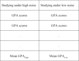
Post facto designs compare group performance on an outcome measure after group differences have already taken place. These designs can be correlational or comparative depending on how the researcher relates one set of scores to the other (i.e., using correlation or difference methods, respectively). A post facto design compares conditions with one another to detect differences in outcome measures. Thus, for example, rather than perform an experiment to detect the impact of noise on human learning, we might ask a sample of students to indicate how loud their music is when they study, and ask them to record their grade point average (GPA). Then we could separate the students into two groups (high and low noise studiers) and compare their GPA measures.
In this design, therefore, we would not manipulate the noise measure; we would simply create groups on the basis of already existing differences in noise conditions. If the outcome measure (GPAs) was different between the groups, we would conclude that noise would possibly be a contributing factor to GPA. We could not speak causally about noise, since many other aspects of studying may have affected GPA (for example, sleep deprivation, studying in groups, caffeine consumption, etc.). Figure 15.2 shows how the post facto design might appear using the noise research question. We would simply use an independent t test to compare the GPA measures for high and low noise studiers.
Figure 15.2 The post facto comparison for independent t test.
This same design could use dependent samples if we deliberately stacked the two samples to be the same on some issue. For example, we might equate the numbers of women and men students as well as ensure equivalent numbers of freshmen, sophomores, juniors, and seniors in both noise groups. If we did this, we would be matching the groups and therefore creating dependent samples. Under these circumstances, we would need to use the dependent t test.
In the independent t test, the researcher compares a pair of samples to see whether these can be said to belong to a common population. The experimental and post facto designs that we discussed earlier would both yield sample data for two samples. Figure 15.3 shows how the two sample process works.
Figure 15.3 The independent t test process.
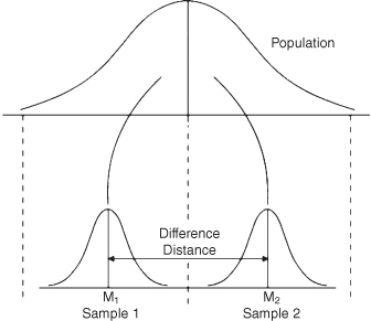
The chief concern with this test is the difference in the means of the two samples. If the samples are chosen randomly, by chance the means will both be close to the actual population mean (the value of which is unknown). By chance alone, the difference between the means should be fairly small.
If we chose two sample groups (or, in an experiment, if we randomly chose a group and randomly assigned them to two groups), we would expect the group means to be similar. In research, we start with this assumption but observe whether the two sample means are still equal after an experimental treatment or if the group means are different when we compare different conditions of the research variable.
Using our previous post facto example above, this would be our reasoning:
But how large does this difference have to be before it could be said that a difference that large could not reasonably be explained by chance and therefore the two groups do not represent a single population? That is the nature of the t test process that we will examine using data from the General Social Survey (GSS).
As an extended example of the independent t test, we will use data from the 2010 GSS database. We can use questionnaire items that related to the issue of general health and work. One of the theoretical questions that we have pursued in several places in this book is whether individual health is in any way connected to the structure and experience of work.
In this example, we use two GSS items to address the research question of whether a person’s perceived health is affected by their judgment of the “fairness” of their earnings. Obviously, the larger research question can be answered in many ways. We are choosing to operationally define the variables (health and fairness) by the GSS respondents’ answers to two questionnaire items. Different studies might use other methods of operationalization, perhaps obtaining an objective measure of health (e.g., electrocardiogram reading) from workers who have either publicly voiced their concern over earnings fairness or not. Providing confidence in the larger issue of concern (health and fairness) can therefore come from a variety of research studies. We are choosing this method to describe the independent t test and how to interpret the findings.
The GSS contains two questions that we will use as the basis of our example:
In order to use SPSS to assist us with the t test for the example, we use the Analyze button in the top menu ribbon and specify Compare Means and Independent Samples T Test as shown in Figure 15.4. When we make this choice, another window appears as shown in Figure 15.5.
Figure 15.4 Using SPSS specification windows for the independent t test.
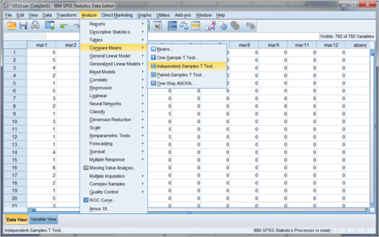
Figure 15.5 Specifying the t test between GenHealth and deserveearn.
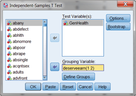
The choices for the t test in Figure 15.5 show that GenHealth is the Test Variable (outcome) and deserveearn is the predictor variable with two categories (1 and 2). You can choose the variables for the analysis from the window on the left side of the panel by using the arrow buttons in the middle of the screen. With this test example, you can simply choose OK at this point, and SPSS will complete the t test analysis.
Figures 15.6 and 15.7 show the SPSS results of the t test analysis of the example variables where the mean of GenHealth is compared between categories of deserveearn. The first panel shown in Figure 15.6 indicates the GenHealth group means for both categories of deserveearn. As you can see, the Less Than Deserved group indicates a lower GenHealth mean than the As Much As or More Than Deserved group. The group mean differences (0.2331) do not appear to be large, but the statistical analysis will determine whether the difference is a significant (nonchance) difference.
Figure 15.6 The t test group means for the example problem.

Figure 15.7 The t test omnibus findings for the example problem.
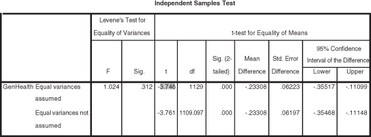
Figure 15.7 shows the statistical analysis of the difference in GenHealth means between the two categories of deserveearn. As you can see (shaded), the T ratio of −3.746 is significant as indicated by the 0.000 figure in the Sig. (2-tailed) column. The T ratio is a negative figure because SPSS entered the value for group 2 (the higher mean value) after group 1. Thus the perceived general health of GSS respondents is higher for those workers who indicated that their earnings were at least as much as they deserved.
Effect size is very important, as we have indicated in earlier sections. There are several ways to calculate effect size for the t test, including the following (Cohen 1988):

We can judge the magnitude of the effect size (d) using the following criteria:

In this example our effect size is judged to have a small effect. Therefore, even though the perceived health is different between groups of deserveearn, it is a small difference. In the world of research, however, even a small effect size difference can be meaningful.
If you are interested in developing a working knowledge of using SPSS for independent t tests, consult a more comprehensive statistical work (e.g., see Abbott 2011). This pursuit will include discussions of the assumptions for the test, how to use SPSS to provide information for the test assumptions, and alternative procedures to use when the assumptions have been violated (e.g., Mann-Whitney U test).
Notes
1 Parts of this section are adapted from M. L. Abbott, Understanding Educational Statistics Using Microsoft Excel® and SPSS® (Wiley, 2011), by permission of the publisher.
2 Some researchers use these kinds of data (ordinal questionnaire items) routinely in survey research, but the procedure is contested by other researchers. The former argue that (even single) items like these from the GSS are commonly used and exhibit many of the properties of interval data. The latter researchers might argue that the questionnaire data are ordinal data and should not be used with parametric procedures. While researchers should be cautious, we take the former position that GSS data have been used meaningfully in similar research and are appropriately used when additional procedures support their use in this fashion. In this example, a separate nonparametric test (Mann-Whitney U test) confirms the parametric (t test) results that are presented and discussed below.
3 See Data Management Unit B, “Using SPSS to Recode t Test,” for an explanation of how we used SPSS to recode variables.