CHAPTER 2

Climate Change from the Globe to California

Michael D. Mastrandrea and William R. L. Anderegg

Abstract. Projections of future anthropogenic climate change derive from global models of the atmosphere, ocean, and land surface known as General Circulation Models (GCMs). Such models provide output at the scale of 100–200 km boxes, but techniques known as “downscaling” can generate projections at higher spatial resolutions. Downscaling can be done via two very different approaches, statistical and dynamic, and like global projections it must rely on trajectories of future greenhouse gas emissions known as emission scenarios. Projections of temperature change in California are largely consistent across models, but changes in precipitation and extreme events are more difficult to model and are also very relevant to the state’s flora and fauna.

---

INTRODUCTION

California’s climate regions range from the coastal, moist redwood forests in the north to the high mountainous regions of the Sierras to the arid deserts of southern California. Over time, the state’s communities and economy have developed strategies to manage climate stresses and to prosper within the state’s diverse climatic zones. Likewise, California’s native flora and fauna have thrived in this variety of climatic regions, making the state one of the world’s most important biodiversity hotspots of species found nowhere else (Myers et al. 2000).

However, the rapidly changing climate is now threatening to exceed the limits of species’ natural strategies for managing climate conditions. While the effects of changing climate on ecosystems have already been noted in California, future changes may overwhelm ecosystems’ natural resilience and cause widespread change. In northern California, the Bay checkerspot butterfly (Euphydryas editha bayensis) became the first documented species driven locally extinct by changing climate (McLaughlin et al. 2002). Looking ahead, future temperature changes could threaten up to 66% of California’s unique plants with greater than 80% range reduction (Loarie et al. 2008). Temperature changes are expected to drive large shifts in bird ranges, leading to entirely new and no-analogue bird communities (Stralberg et al. 2009). These consequences highlight the vulnerability of California’s natural systems to climate variability and change.

Climate modeling and projections of future climate change at the global and regional scale can be used to inform policy decisions to mitigate future climate change by reducing emissions of greenhouse gases, and are a key component of anticipating and managing future risks of climate change through adaptation. In this chapter, we provide an overview of climate modeling and how regional climate projections are produced by downscaling the results of General Circulation Models (GCMs). We discuss climate change scenarios for California, highlighting potential interaction with the state’s ecosystems, and touch briefly on how these might be used in state and regional planning efforts in the future.

PROJECTING GLOBAL CLIMATE

Climate projections depend in large part on two factors: (1) How much and how quickly greenhouse gases are emitted into the atmosphere and (2) how the climate, oceans, and terrestrial systems respond to rising atmospheric concentrations of these gases.

Emission Scenarios

In 2000 the Intergovernmental Panel on Climate Change (IPCC) Special Report on Emission Scenarios (SRES) developed the most commonly used set of future emission scenarios based on different assumptions about global development paths (Nakicenovic et al. 2000). Scenarios differ in their trajectories for population and economic growth, technological development, and patterns in trade and sharing of technologies, among other things. Each scenario represents a possible “baseline” trajectory of emissions without explicit policy intervention, although some scenarios are more likely to simulate expected “business as usual” trends with continued high emissions and others are closer to a pathway that could be achieved with a stringent emissions reduction policy.

These scenarios are now over 10 years old, and a new set of emission scenarios and climate change projections are now available for use in climate impacts and policy analysis, based on the Representative Concentration Pathways (RCPs) (Moss et al. 2010, Collins et al. 2013). One primary difference is that the RCPs include trajectories that assume policy interventions, yielding a wider range of possible futures. Figure 2.1 compares SRES and RCP scenarios in terms of radiative forcing, a measure of the strength of the warming influence on the climate system from increased atmospheric greenhouse gas concentrations under each emission scenario. A growing number of analyses employ the RCPs, but much of the published literature on climate impacts still relies on the SRES scenarios, including climate and impact projections for California. Thus, we focus in this chapter on the SRES scenarios.

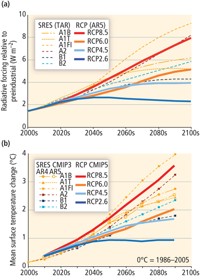
FIGURE 2.1: Range of SRES and RCP emission scenarios. Comparison of projected radiative forcing and temperature trajectories under the SRES and RCP scenarios. Source: Burkett et al. (2014).

These scenarios are run in global GCMs to produce projections of global and regional climate change. GCMs are developed by different research groups around the world and represent many different ways to simulate complex interactions between the atmosphere, ocean, ice sheets, and land surface that determine the sensitivity of the earth system to increasing greenhouse gas concentrations.

Climate Sensitivity

Climate sensitivity is a measure of how much temperatures will rise with a given increase in atmospheric greenhouse gas concentrations. Climate sensitivity is not known with certainty, as it depends on how various earth system processes respond to warming and on various “feedbacks” that either amplify or dampen warming. Scientific understanding of exactly how these processes and feedbacks will interact is still developing. For example, as temperatures rise, the atmosphere can hold more water vapor. More atmospheric water vapor traps heat and increases global temperatures further—a positive feedback. However, the clouds created by this water vapor could either enhance warming by absorbing and radiating outgoing infrared radiation from the earth’s surface (another positive feedback) or dampen warming by reflecting more incoming shortwave radiation from the sun back to space before it reaches the earth’s surface (a negative feedback).

The “climate sensitivity” represents the response of the climate system to changes in CO₂, and this sensitivity is often expressed as the long-term temperature increase associated with a doubling of atmospheric CO₂ concentrations. The IPCC reports a likely range for climate sensitivity of 1.5–4.5°C (2.7–8.1°F) meaning at least a 66% probability that the climate sensitivity is within this range (Collins et al. 2013). The IPCC also concludes that the climate sensitivity is extremely unlikely to be less than 1°C (meaning less than 5% probability) and very unlikely to be more than 6°C (meaning less than 10% probability). Different climate models treat the relevant processes and feedbacks differently, which leads to a range of values for climate sensitivity exhibited across models.

Therefore, different models project different levels of global temperature increase even for the same emission scenario, which can serve as an estimate of the uncertainty in the climate system’s response to the same greenhouse gas forcing. The projections for the end of the century that follow illustrate this spread across models.

The Projections

Over the next few decades, the projected changes in global mean temperature are fairly similar across emission scenarios due to the inertia of the climate system (Meehl et al. 2007, Collins et al. 2013). By the second half of the century, however, different emission scenarios yield vastly different temperature responses. These characteristics are illustrated in Figure 2.2 for the SRES scenarios. For the highest-emission scenario (A1FI), models project global average warming of 2.4–6.4°C (4.3–11.5°F) by the end of the century (Meehl et al. 2007). For the lowest-emission scenario (B1), models project warming of 1.1–2.9°C (2–5.2°F) by the end of the century. The difference between these ranges indicates the influence of different emission trajectories on projected climate change. The ranges themselves represent uncertainties associated with how models handle the response of the climate system captured in the climate sensitivity, and how the uptake of carbon dioxide by the ocean and by land ecosystems will be altered by changing temperature and atmospheric greenhouse gas concentrations.

FIGURE 2.2: Projected global average temperature increase through the 21st century under several emission scenarios. The left-hand panel shows the evolution of temperature increase over time (as well as projected temperature increase assuming constant year-2000 atmospheric greenhouse gas concentrations). The right-hand panel shows the ranges of temperature increase at the end of the century (across different climate models) for six emission scenarios. Source: IPCC (2007).

A significant fraction of current greenhouse gas emissions are taken out of the atmosphere by oceanic processes and living plants. The strength of these ocean and land carbon “sinks” is expected to decrease over time, leaving a greater fraction of emissions in the atmosphere to drive further warming. Effects of climate change such as severe drought may also contribute to the switching of land ecosystems from a carbon sink to a carbon source. For example, a recent study found declines between 2000 and 2009 in the amount of global terrestrial ecosystem productivity (carbon uptake), driven by regional drought (Zhao and Running 2010).

Downscaling

Most global climate models are currently limited to representing the earth’s surface with “grid cells” of roughly 100–200 km on a side. Climatically important phenomena, such as clouds, occur on much smaller scales, and some areas, including California, have complex topography that cannot be adequately represented at this coarse scale. Projections for precipitation, for instance, are hindered by this lack of spatial detail, that, for example, cannot fully distinguish the moist western side of the Sierras from the much drier eastern side. Indeed, many simulations of the current climate have identified differences in some regions between modeled and observed conditions. Scientists use a variety of tools to address these differences by “downscaling” results from global models to a regional scale. It is important to note that while generating projections at a finer spatial scale, downscaling does not necessarily lead to greater confidence or accuracy in those projections.

Downscaling techniques generally fall into two categories—dynamic and statistical—and various forms of each method involve different trade-offs in feasibility and model complexity and accuracy. Dynamical downscaling techniques employ a regional climate model running at a finer resolution than global models. These Regional Circulation Models (RCMs) use dynamic and time-varying inputs from atmospheric GCMs as their boundary conditions at the edge of the region of interest. They can be constructed as a one-way nesting within the GCM (inputs travel only from the GCM into the RCM) or with two-way nesting (feedback and inputs move back and forth between the two models). All downscaling techniques must be validated against independent data (not used in constructing the model) and dynamic techniques are usually validated with present-day reanalysis data (Wigley 2005). In essence, the RCM is given a set of boundary conditions in the past, then run up to present day. The model’s results are compared to an independent reanalysis of modern-day climate observations. How well the RCM reproduces observed climate trends within its region is of crucial importance for model accuracy. Chief among its disadvantages, dynamic downscaling is computationally intensive, which then limits the feasibility for running a large number of long-term projections under different emission scenarios or using different GCMs as boundary conditions.

Much of the downscaling conducted to date in California has used statistical techniques to downscale GCM projections (Wood et al. 2004, Cayan et al. 2008a, Cayan et al. 2012). The general goal is to develop various transfer functions (statistical relationships) that can be used to link coarse-scale (e.g., 200-km grid boxes) data from GCMs to finer-scale (e.g., 12-km grid boxes) future projections. Statistical downscaling as applied in California has used two approaches. The first, Bias Correction and Spatial Downscaling (BCSD), links observed climate patterns with the patterns represented in global climate model simulations of the same historical period. Distributions of temperature and precipitation for each calendar month are assembled for observed data (e.g., covering 1950–1999). Distributions of the same time period are also assembled from GCM simulations for each grid box, and compared to the observed distributions. Differences in the GCM mean and variance for the historical period at the individual sites are corrected and the same corrections are then applied to future GCM projections. The model is then run for the future and projections can be made on a variable- and site-specific basis. For example, a GCM projection for total precipitation in January of 2050 in a certain grid box is compared to the distribution of total January precipitation values simulated by the GCM for that grid box during the observed period (e.g., 1950–1999). The projected total precipitation will correspond to a certain percentile in that distribution (e.g., the median). In this example, the total precipitation for January in each downscaled area within that particular grid box would be set to the median value of the observed distribution of January precipitation for that downscaled area (Wigley 2005, Cayan et al. 2008a).

The BCSD approach preserves the statistical distribution of temperature and precipitation, but does not yield time series that match the daily progression of weather simulated by the GCM (Maurer et al. 2010, Cayan et al. 2012). The second approach, Bias-Corrected Constructed Analogues (BCCA), preserves the daily evolution of weather that is simulated by the GCM. It combines the initial large-scale bias correction step of BCSD, applied at a daily scale, with a different approach to spatial downscaling. In BCCA, each day of the GCM simulation is compared with a library of observed coarse-scale and corresponding finer-scale daily patterns of the variable of interest (e.g., temperature, precipitation). The 30 coarse-scale observed patterns that are most similar to the simulated day are selected, and a linear combination of these patterns is used to produce a coarse-resolution analogue. The same linear combination is then applied to the corresponding 30 finer-scale patterns to produce the downscaled projection.

Statistical downscaling relies on the fundamental assumption that past spatial and temporal relationships between the climate and area modeled will remain constant in the future. Such relationships may change as the climate changes (Meehl et al. 2000, Alley et al. 2003). Statistical downscaling is much less computationally intensive and more tractable than dynamic downscaling, and is therefore more feasible for long-term projections under multiple emission scenarios. Both statistical and dynamic downscaling methods have been found to be capable of reproducing accurate characterizations of both the mean and variance of known climatic events (Wigley 2005).

CALIFORNIA’S CHANGING CLIMATE

In recent decades, California and the western United States have experienced clear signs of a changing climate. Average temperatures for the state of California have risen about 0.9°C (1.7°F) from 1895 to 2011, sea level has risen more than half a foot, spring snow levels in lower- and mid-elevation mountain areas have dropped and snowpack melting has shifted earlier, flowers are blooming one to two weeks earlier, and warmer temperatures combined with long dry seasons over the last few decades have contributed to more severe wildfires (Cayan et al. 2008a, Cayan et al. 2012, Moser et al. 2012, Garfin et al. 2014). California’s climate is expected to change considerably over this century. The severity of these changes depends on the rate at which greenhouse gases accumulate in the atmosphere based on policy and development choices and how the climate responds to the rising concentrations of these gases. Projected changes include further increases in average temperatures, changes in precipitation patterns, rising sea levels, and changes in the frequency and/or severity of extreme events such as heat waves, droughts, and fires.

Temperature

By mid-century, the average annual temperature of California is projected to rise ∼1–3°C (∼1.8–5.4°F) above the 1961–1990 average, regardless of the emission scenario evaluated (Cayan et al. 2012, Moser et al. 2012). By the end of the century, temperatures in California are projected to rise ∼2.5–4.8°C (4.6–8.6°F) under the medium-high A2 scenario. Holding emissions to the lower B1 pathway would still lead to warming of ∼1.5–3.3°C (2.8–6°F). The divergence of projections for higher- and lower-emission scenarios by the end of the century demonstrates the long-term benefits of mitigation policy.

The rise in average annual temperature has very different implications for seasonal temperatures. In the past five decades, spring and winter temperatures have increased more than the annual average, while summer temperatures have increased more slowly. In contrast, studies predict that this pattern will reverse in the future, with summer temperatures rising most rapidly (Cayan et al. 2008a, Cayan et al. 2012). By the end of the century, summer temperatures are projected to rise 1.5–6°C (2.7–10.8°F), while winter temperatures are projected to rise 1–4°C (1.8–7.2°F) across the higher- and lower-emission scenarios. Inland temperatures are also projected to rise faster than coastal temperatures, due to the stabilizing influence of the ocean.

Rising summer temperatures are particularly of concern in terms of impacts on many ecosystems and species (see Part II of this volume). Coupled climate-vegetation models suggest that alpine and subalpine forests may be strongly affected by rising summer temperatures (Lenihan et al. 2008). Higher summer temperatures also work in conjunction with drought to increase the risk of climate-related disturbances to ecosystems such as wildfires and drought-induced forest die-off (Anderegg et al. 2013).

Precipitation

For California (and more generally), different climate models produce projections of precipitation change that vary far more widely than projections of temperature. Precipitation patterns are influenced by regional topography, proximity to geographical features such as mountains or bodies of water, regional temperature differences, and larger-scale atmospheric circulation patterns. Precipitation often varies widely at scales below the grid-box scale of GCMs. While downscaling methods can also be applied to precipitation, uncertainty regarding projections of precipitation remains higher than for temperature.

Projected changes in total annual precipitation in California over this century vary, but the most prevalent pattern suggested is drier conditions (Cayan et al. 2009, Cayan et al. 2012). No model projections suggest a change in the Mediterranean seasonal pattern of precipitation California currently experiences, with most precipitation falling between November and April.

Warming temperatures are projected to decrease the amount of precipitation falling as snow and increase the amount falling as rain. This pattern is expected to continue the already observed trend of decreased spring snow accumulation in the Sierra Nevada (Kapnick and Hall 2009, Cayan et al. 2012), and lead to earlier spring melting of snowpack. By the 2090s, the amount of water stored as snow on April 1 across the Sierra Nevada is projected to be reduced on average to 25% of its historical (1961–1990) level under the medium-high A2 scenario, and be reduced on average to 51% of historical levels under the lower B1 scenario (Cayan et al. 2012).

Sea Level Rise

Warming temperatures contribute to global sea level rise through two main processes. First, a hotter atmosphere causes the ocean to warm, leading to thermal expansion of ocean water. Second, warmer temperatures melt mountain glaciers and the large ice sheets in Greenland and Antarctica, adding water to the ocean that has been stored on land as ice. In California, records suggest an observed rate of sea level rise of 17–20 cm (6.7–7.9 in) per century, which is similar to the global estimate (Cayan et al. 2012).

The magnitude of future sea level rise depends on the level of future warming, uncertainties in the response of the system to warming, and uncertainties in the rates of ice sheet melting. While sea level rise due to thermal expansion and some components of melting ice can be reliably projected (though not without some uncertainty), the rates of melting of the large ice sheets in Greenland and Antarctica are more uncertain—specifically, in terms of quantifying the rate of discharge of ice from these ice sheets into the surrounding oceans, which has accelerated in recent years. The IPCC Fifth Assessment Report projects the global sea level to rise 45–82 cm (1.5–2.7 ft) by the last two decades of the century for the highest RCP scenario discussed above (RCP8.5; somewhat comparable to A2; see Figure 2.1), 32–63 cm (1–2.1 ft) for RCP4.5 (somewhat comparable to B1) and 26–55 cm (0.9–1.8 ft) for the lowest RCP scenario (RCP2.6; a low-emission mitigation scenario), compared with 1986–2005 (Church et al. 2013). Another analysis based on the observed relationship between temperature increase and the rate of sea level rise over the 20th century suggests a larger range (across the A2 and B1 scenarios) of ∼30–45 cm (1–1.5 ft) by mid-century and 90–140 cm (3–4.6 ft) by the end of the century above 2000 levels (Cayan et al. 2012).

Extreme Events

While changes in average temperature, precipitation, and sea level will very likely occur gradually, the frequency and intensity of extreme events such as heat waves, droughts, and floods can change substantially with even small average changes in temperature or precipitation. Such extreme events can greatly impact natural systems through population crashes or alterations to the physical environment such as flood erosion (Parmesan et al. 2000). Rising average temperature will lead to more frequent and longer periods of extreme heat, and the potential for temperatures above the range of historical experience. For example, in Sacramento, the frequency of extreme temperatures currently estimated to occur once every 50 years (a severe heat wave by current standards) is projected to increase at least tenfold by the end of the century under the higher A2 scenario and fivefold under the lower B1 scenario (Cayan et al. 2012). Additionally, the length of individual events is expected to increase.

Extremes in coastal sea levels are already increasing in many, but not all, parts of California. For example, Crescent City has experienced a slight decrease in the occurrence of extreme sea levels due to coastal uplift along parts of the northern California coast (Cayan et al. 2008b). The occurrence of extreme sea levels has increased 20-fold since 1915 in San Francisco, however, and 30-fold in La Jolla since 1933. With climate change, increasing frequency and duration of sea levels that exceed current extreme thresholds threaten coastal infrastructure and flood defenses that were designed to protect against the historical range of sea levels and storm intensities (Cayan et al. 2008b, Cayan et al. 2012, Moser et al. 2012).

CONCLUSION

California’s diversity in climate regions makes the state vulnerable to changing conditions in many ways. Global models and downscaled regional projections provide a framework for selecting policies to dampen the impacts of future changes in climate. Many such models have been run for California and hold the potential to project future statewide impacts on ecosystems and species (e.g., Loarie et al. 2008, Stralberg et al. 2009) and inform on-the-ground management at individual sites (e.g., Mastrandrea et al. 2010).

Projected trends in temperature and precipitation, as well as sea level rise and changes in the frequency and/or intensity of some types of extreme events, will stress the state’s social and natural systems even under lower-emission scenarios. Concurrent and synergistic interactions between climatic changes (i.e., longer heat waves coupled with more intense summer droughts, fires, etc.) and extreme events present perhaps the largest potential to threaten natural systems in the near future.

LITERATURE CITED

Alley, R. B., J. Marotzke, W. D. Nordhaus, J. T. Overpeck, D. M. Peteet, R. A. Pielke Jr, R. T. Pierrehumbert, P. B. Rhines, T. F. Stocker, L. D. Talley et al. 2003. Abrupt climate change. Science 299:2005–2010.

Anderegg, W. R. L., J. Kane, and L. D. L. Anderegg. 2013. Consequences of widespread tree mortality triggered by drought and temperature stress. Nature Climate Change 3:30–36.

Burkett, V. R., A. G. Suarez, M. Bindi, C. Conde, R. Mukerji, M. J. Prather, A. L. St. Clair, and G. W. Yohe. 2014. Point of departure. In C. B. Field, V. R. Barros, D. J. Dokken, K. J. Mach, M. D. Mastrandrea, T. E. Bilir, M. Chatterjee, K. L. Ebi, Y. O. Estrada, R. C. Genova et al. (eds), Climate Change 2014: Impacts, Adaptation, and Vulnerability. Part A: Global and Sectoral Aspects. Contribution of Working Group II to the Fifth Assessment Report of the Intergovernmental Panel on Climate Change. Cambridge University Press, Cambridge, UK.

Cayan, D. R., E. P. Maurer, M. D. Dettinger, M. Tyree, and K. Hayhoe. 2008a. Climate change scenarios for the California region. Climatic Change 87:21–43.

Cayan, D. R., P. D. Bromirski, K. Hayhoe, M. Tyree, M. D. Dettinger, and R. E. Flick. 2008b. Climate change projections of sea level extremes along the California coast. Climatic Change 87:57–73.

Cayan, D. R., M. Tyree, M. D. Dettinger, H. Hidalgo, T. Das, E. Maurer, P. D. Bromirski, N. Graham, and R. E. Flick. 2009. Climate Change Scenarios and Sea Level Rise Estimates for California: 2008 Climate Change Scenarios Assessment. PIER Report CEC-500-2009-014-F, California Energy Commission, Sacramento, CA.

Cayan, D. R., M. Tyree, D. Pierce, and T. Das. 2012. Climate Change and Sea Level Rise Scenarios for California Vulnerability and Adaptation Assessment. California Energy Commission Report CEC-500-2012-008, California Energy Commission, Sacramento, CA.

Church, J. A., P. U. Clark, A. Cazenave, J. M. Gregory, S. Jevrejeva, A. Levermann, M. A. Merrifield, G. A. Milne, R. S. Nerem, P. D. Nunn et al. 2013. Sea level change. In T. F. Stocker, D. Qin, G.-K. Plattner, M. Tignor, S. K. Allen, J. Boschung, A. Nauels, Y. Xia, V. Bex, and P. M. Midgley (eds), Climate Change 2013: The Physical Science Basis. Contribution of Working Group I to the Fifth Assessment Report of the IPCC. Cambridge University Press, Cambridge, UK.

Collins, M., R. Knutti, J. Arblaster, J.-L. Dufresne, T. Fichefet, P. Friedlingstein, X. Gao, W. J. Gutowski, T. Johns, G. Krinner et al. 2013. Long-term climate change: Projections, commitments and irreversibility. In T. F. Stocker, D. Qin, G.-K. Plattner, M. Tignor, S. K. Allen, J. Boschung, A. Nauels, Y. Xia, V. Bex, and P. M. Midgley (eds), Climate Change 2013: The Physical Science Basis. Contribution of Working Group I to the Fifth Assessment Report of the IPCC. Cambridge University Press, Cambridge, UK.

Garfin, G., G. Franco, H. Blanco, A. Comrie, P. Gonzalez, T. Piechota, R. Smyth, and R. Waskom. 2014. Southwest. Chapter 20. In J. M. Melillo, Terese (T. C.) Richmond, and G. W. Yohe (eds), Climate Change Impacts in the United States: The Third National Climate Assessment. U. S. Global Change Research Program, Washington, DC. 462–486. doi:10.7930/J08G8HMN.

IPCC. 2007. Summary for policymakers. In S. Solomon, D. Qin, M. Manning, Z. Chen, M. Marquis, K. B. Averyt, M. Tignor, and H. L. Miller (eds), Climate Change 2007: The Physical Science Basis. Contribution of Working Group I to the Fourth Assessment Report of the IPCC. Cambridge University Press, Cambridge, UK.

Kapnick, S. and A. Hall. 2009. Observed Changes in the Sierra Nevada Snow Pack: Potential Causes and Concerns. PIER Technical Report CEC-500-2009-016-F, California Climate Change Center, Santa Barbara, CA.

Lenihan, J. M., D. Bachelet, R. P. Neilson, and R. Drapek. 2008. Response of vegetation distribution, ecosystem productivity, and fire to climate change scenarios for California. Climatic Change 87:S215–S230.

Loarie, S. R., B. E. Carter, K. Hayhoe, S. McMahon, R. Moe, C. A. Knight, and D. D. Ackerly. 2008. Climate change and the future of California’s endemic flora. PLOS ONE 3(6):e2502. doi:10.1371/journal.pone.0002502.

Mastrandrea, M. D., N. E. Heller, T. L. Root, and S. H. Schneider. 2010. Bridging the gap: Linking climate-impacts research with adaptation planning and management. Climatic Change 100:87–101.

Maurer, E. P., H. G. Hidalgo, T. Das, M. D. Dettinger, and D. R. Cayan. 2010. The utility of daily large-scale climate data in the assessment of climate change impacts on daily streamflow in California. Hydrology and Earth System Sciences 14:1125–1138.

McLaughlin, J. F., J. Hellman, C. Boggs, and P. R. Ehrlich. 2002. Climate change hastens population extinctions. Proceedings of the National Academy of Sciences of the United States of America 99:670–674.

Meehl, G. A., F. Zwiers, J. Evans, T. Knutson, L. Mearns, and P. Whetton. 2000. Trends in extreme weather and climate events: Issues related to modeling extremes in projections of future climate change. Bulletin of American Meteorological Society 81:427–436.

Meehl, G. A., T. F. Stocker, W. D. Collins, P. Friedlingstein, A. T. Gaye, J. M. Gregory, A. Kitoh, R. Knutti, J. M. Murphy, A. Noda et al. 2007. Global climate projections. In S. Solomon, D. Qin, M. Manning, Z. Chen, M. Marquis, K. B. Averyt, M. Tignor, and H. L. Miller (eds), Climate Change 2007: The Physical Science Basis. Contribution of Working Group I to the Fourth Assessment Report of the IPCC. Cambridge University Press, Cambridge, UK.

Moser, S., J. Ekstrom, and G. Franco. 2012. Our Changing Climate 2012: Vulnerability & Adaptation to the Increasing Risks from Climate Change in California. California Energy Commission Report CEC-500-2012-007, California Energy Commission, Sacramento, CA.

Moss, R. H., J. A. Edmonds, K. A. Hibbard, M. R. Manning, S. K. Rose, D. P. van Vuuren, T. R. Carter, S. Emori, M. Kainuma, T. Kram et al. 2010. The next generation of scenarios for climate change research and assessment. Nature 463:747–756.

Myers, N., R. A. Mittermeie, C. G. Mittermeier, G. A. B. de Fonseca, and J. Kent. 2000. Biodiversity hotspots for conservation priorities. Nature 403:853–858.

Nakicenovic, N., J. Alcamo, G. Davis, B. de Vries, J. Fenhann, S. Gaffin, K. Gregory, A. Grübler, T. Y. Jung, T. Kram et al. 2000. IPCC Special Report on Emission Scenarios. Cambridge University Press, Cambridge, UK.

Parmesan, C., T. L. Root, and M. R. Willig. 2000. Impacts of extreme weather and climate on terrestrial biota. Bulletin of the American Meteorological Society 81:443–450.

Stralberg, D., D. Jongsomjit, C. A. Howell, M. A. Snyder, J. D. Alexander, J. A. Wiens, and T. L. Root. 2009. Re-shuffling of species with climate disruption: A no-analog future for California birds? PLOS ONE 4:e6825.

Wigley, T. M. L. 2005. Input Needs for Downscaling Climate of Climate data. California Energy Commission Discussion Paper.

Wood, A. W., L. R. Leung, V. Sridhar, and D. P. Lettenmaier. 2004. Hydrologic implications of dynamical and statistical approaches to downscaling climate model outputs. Climate Change 62:189–216.

Zhao, M. and S. Running. 2010. Drought-induced reduction in global terrestrial net primary production from 2000 through 2009. Science 329:940–943.