11
The Wine Consumer and Demand
According to the Wine Market Council, there are one hundred million wine consumers in the United States. About eleven million of these drink wine every day, another forty-five million consume wine at least once a week, and the rest typically imbibe a couple of times a month. A typical American wine consumer drinks about thirty-five bottles of wine per year or three and one-half five-ounce glasses per week. In the aggregate, wine consumers in the United States drink the equivalent of 295 million cases of wine per year, the largest total consumption of any nation in the world, but per capita consumption is still much less than in many other countries, such as France, Italy, Spain, and the United Kingdom.1 This chapter begins by describing the characteristics of these wine consumers and trends and patterns of wine consumption in the United States. Economic concepts are then used to shed light on wine consumers’ behavior and to analyze important factors that affect wine consumption.
CHARACTERISTICS OF WINE CONSUMERS
Sixty-six percent of American adults aged twenty-one or older choose to consume alcoholic beverages.2 Forty-four percent drink wine; some of these also consume beer or spirits. A typical wine consumer tends to be an affluent, college-educated, middle-aged, married, homeowner in a technical, professional, or proprietary occupation, and enjoys cultural events and participating in sports or exercise-related activities. A majority of wine drinkers have household incomes in excess of $100,000, about half have college degrees, more than one-third have graduate degrees, and almost nine out of ten own their own homes. About half of all wine drinkers are between the ages of thirty-five and fifty-five, and more women consume wine than men. Wine is the preferred alcoholic beverage of women aged thirty and older, and the proportion who choose wine over beer and spirits increases with age. While more than half of all American women older than thirty prefer to drink wine, more than 80 percent of men of all ages prefer beer or spirits. However, men tend to drink more of any type of alcoholic beverage than women.
Most wine is consumed by a relatively small segment of the U.S. population. Frequent wine consumers, those who drink wine at least once a week, represent 25 percent of the adult population, but account for 93 percent of the wine consumed. About 20 percent of these drink wine every day. Consumption of wine on a daily basis increases with age. Only 6 percent of Americans aged from twenty-one to thirty-four drink wine each day, while 12 percent of those sixty-five or older do so daily. Infrequent wine consumers, those who drink wine at least once a month, constitute 19 percent of the adult population and account for only 7 percent of the quantity of wine consumed. A typical infrequent consumer drinks wine two to three times a month.
A large study by Constellation Brands, called Project Genome, suggests that there are significant individual differences among U.S. consumers in their attitudes to wine. The largest segment, 23 percent, report being overwhelmed when making wine-buying decisions. This is largely the result of the vast number of wines from which they must choose and lack of information about the relevant characteristics of these products. The second-largest segment, comprising 20 percent of wine consumers, see wine as a status symbol and believe that price is a good index of quality. A typical wine “image seeker” tends to be a male in his mid-thirties. Another 16 percent of wine consumers have a strong preference for well-known, national brands and tend to be loyal to a particular brand. Fourteen percent of wine consumers are relatively uninformed about wine and tend to have a few favorite wine brands that they purchase on a regular basis. The smallest segment of wine consumers, 12 percent of the wine-drinking population, are very enthusiastic and knowledgeable about wine and keep abreast of critics’ evaluations and quality ratings. About half of all wine expenditures are made by wine enthusiasts or status-conscious individuals, accounting for one-third of all U.S. wine consumers.
TRENDS AND PATTERNS IN WINE CONSUMPTION
This section discusses some notable trends and patterns in wine consumption in the United States. The focus is on aggregate sales and expenditures, quantity consumed, and price. Some information on the types of wine and share of wine consumed in different price segments is also provided.
Wine Sales and Expenditures
To describe the behavior of aggregate wine sales data, it is useful to begin with the accounting identity S = PQ. S is the dollar value of wine sales during a given period of time or equivalent dollar value of consumer wine expenditures. P is the average price per unit of wine for the time period. It is sometimes called the nominal price, because it is an absolute measure of price in current dollars. Q is the number of units of wine purchased by consumers during the given period. Units of wine are typically measured in gallons, 750 ml bottles, or twelve-bottle cases. This identity informs us that consumer spending on wine can increase (decrease) if consumers pay a higher (lower) price for the same quantity of wine, purchase a larger (smaller) quantity of wine at the same price, or some combination of these. An increase (decrease) in the average price of wine can result from an increase (decrease) in the general level of prices in the economy or inflation (deflation), an increase (decrease) in the price of wine relative to the prices of other goods and services, an improvement in wine quality, or consumers substituting higher-priced (lower-priced) wine products for lower-priced (higher-priced) ones. For example, if the inflation rate for a given year is 5 percent and the average price of wine increases by 7 percent, the relative price of wine has increased by 2 percent. This 2 percent increase in relative price can be the result of an increase in demand for wine relative to supply or a manifestation of consumers’ willingness to pay a higher price for higher-quality wine, which may result from either a general improvement in the quality of wine products or consumers substituting higher-priced premium wine for lower-priced commodity wine.
Table 1 provides data on several alternative measures of annual sales of wine in the United States over the twenty-year period 1991 through 2010, for which reliable sales data are available. Current dollar (nominal) expenditures on wine grew from $10.9 billion in 1991 to $30 billion in 2010, an increase of 175 percent. Aggregate spending on wine increased each year between 1994 and 2007, before declining in both 2008 and 2009. Part of the increase in wine expenditures during this period is the result of an increase in the average level of prices of all goods, as well as an increase in the population of potential wine consumers. Column 3 of table 1 adjusts nominal spending for inflation and provides a measure of real wine sales in year 2010 dollars. The pattern in real spending mirrors that of nominal spending; however, after accounting for inflation, real spending for the period 1991 to 2010 increased by only 72 percent. Column 4 makes an additional adjustment for population growth and measures real spending on a per capita basis. In 1991, spending per U.S. resident on wine measured in 2010 dollars was $69. By 2010, it had grown to $97, an increase of 41 percent. This indicates that the pattern of rising expenditures persisted even after accounting for population growth and inflation. The last column in table 1 gives a measure of wine expenditures as a percentage of consumer disposable income. During this twenty-year period consumers devoted roughly the same proportion of disposable income to wine. In 1991, a typical consumer spent 0.25 percent of after-tax income on wine. By 2010, this had increased slightly to 0.26 percent.
TABLE 1U.S. ANNUAL WINE SALES, 1991–2010

The pattern of rapidly rising nominal and real spending on wine occurred during a period of economic expansion and rising disposable income, and persisted during a brief, mild recession from March to November 2001. However, this trend was interrupted shortly after the onset of the major economic recession in December 2007. Not only did consumers reduce total spending on wine, but they also devoted a smaller portion of their reduced disposable income to wine. This recession, which was the biggest economic contraction in sixty-five years, officially ended in June 2009. It appears that the upward trend in wine expenditures may have once again returned as consumers increased spending on wine in 2010.
The data on the year-to-year behavior of wine expenditures masks the seasonal pattern that occurs with regularity within any given year. In a typical year, monthly wine sales display relatively little variation between January and October. However consumer spending on wine increases dramatically during the months of November and December, largely because of the holiday season that includes Thanksgiving, Christmas, and New Year. For example, in 2011, monthly off-premises wine sales varied within a range of $675 to $750 million during the first ten months of the year, but exceeded $900 million for November and December.
Quantity of Wine Consumed
Table 2 presents annual data on the quantity of wine consumed per capita in the United States, measured in gallons, for the period 1951 to 2010. Between 1952 and 1962, the amount of wine consumed per capita was flat, varying within a range of 0.88 to 0.94 gallons. Beginning in 1963, per capita consumption rose continuously for two decades, reaching a peak of 2.43 gallons in 1986. The quantity of wine consumed per resident during this twenty-three-year period increased at an annual average rate of 7.4 percent and was 2.7 times higher in 1986 than 1963. However, per capita consumption then proceeded to decline each year until it hit a low of 1.74 gallons in 1993, the same quantity of wine a typical member of the U.S. population had consumed in 1976. In 1994, per capita consumption started to rise once again, and it increased each year, with the exception of 2000, achieving an historic high of 2.54 gallons per resident in 2010.
TABLE 2U.S. WINE CONSUMPTION PER CAPITA, 1951–2010 (GALLONS)


For the most part, per capita wine consumption has been resistant to economic downturns. During this fifty-year year period, the economy experienced ten economic recessions with declining aggregate output and income. However, the quantity of wine consumed per resident fell during only two of these contractions in economic activity. During the 1973–75 recession, when oil prices skyrocketed, inflation continued unabated, and the stock market fell precipitously, wine consumption per capita increased by 12 percent. Even during the recent severe recession of 2007–9, per capita consumption rose by a healthy 1.2 percent. However, during this same recessionary period, nominal wine expenditures decreased from $106 to $95 per capita, a decline of about 10.4 percent. The contemporaneous increase in the quantity of wine consumed and decrease in spending on a per capita basis indicates that consumers were paying a lower average price for the wine they purchased. The evidence suggests that the average price of a bottle of wine fell for two reasons. First, many wine firms lowered prices in response to the poor economic environment in order to sell their wine. Second, a number of consumers maintained or increased their consumption of wine, but substituted lower-priced commodity and premium wines for the higher-priced luxury wines they were consuming prior to the downturn, when they had higher incomes and there was less uncertainty about their employment status.
Even though wine consumption per capita is at an historic high in the United States, we still consume significantly less wine per resident than many other nations, such as France (12 gal.), Italy (11 gal.), Spain (7 gal.), Australia (6.6 gal.), Argentina (6.3 gal.), the United Kingdom (5.7 gal.), and Canada (2.6 gal.), to name just a few of the thirty-two countries that consume more wine per resident than the United States.3
Wine Prices
Table 3 reports several alternative measures of the average price of a bottle of wine in the United States for the period 1991 to 2010. To calculate the nominal price shown in column 2 of the table, I use the accounting identity, S = PQ, and the available data on aggregate nominal wine sales (S) and total gallons consumed (Q). Gallons are converted to 750 ml bottles and price is expressed as dollars per bottle. This measure of price will change if either the prices of wine products change or the distribution of wine purchases at various price points change. For instance, the average price of wine will decrease if the prices of all wine products remain unchanged, but consumers purchase more lower-priced and fewer higher-priced products.
TABLE 3U.S. ANNUAL AVERAGE PRICE OF WINE PER 750 ML BOTTLE, 1991–2010
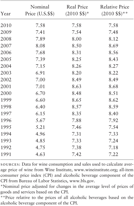
During this twenty-year period, the nominal price of wine increased in sixteen years and fell in only four. In 2010, the average price of a bottle of wine at $7.58 was 64 percent higher than in 1991, when consumers paid $4.63. However, we would like to know whether wine prices have been rising more or less rapidly than the prices of other goods and services in general, and the prices of alcoholic beverages in particular. Column 3 of Table 3 reports a measure of the real price of wine expressed in year 2010 dollars, which adjusts the nominal price for changes in the average level of prices of goods and services using the all-item consumer price index (CPI). The real price of wine rose in ten and declined in ten years. After adjusting for inflation, the price of wine increased by a mere 2.2 percent over this twenty-year period, indicating that almost all of the increase in nominal price can be attributed to inflation. Moreover, it is generally recognized that significant improvements were made in wine quality during this period, so one may easily argue that after adjusting for the higher quality of wine products, wine has become a “better bargain” relative to many other goods and services.
For many consumers, beer and spirits substitute for wine. When the price of wine changes relative to the price of these substitute alcoholic beverages, some consumers are induced to purchase more of the beverage whose price is relatively lower and less of the one whose price is comparatively higher. Column 4 reports a measure of the price of wine relative to the prices of all alcoholic beverages using the alcoholic beverage component of the CPI. Once again this relative price is in 2010 dollars. The behavior of relative price shows that the price of wine increased relative to the price of all alcoholic beverages in thirteen years and decreased in seven. By 2010, the price of wine was 5 percent higher than prices of other alcohol beverages relative to 1991. Once again, one can argue that consumers were more than compensated for this rather small increase in relative price because of the bigger improvement in wine quality compared to beverages like beer and spirits.
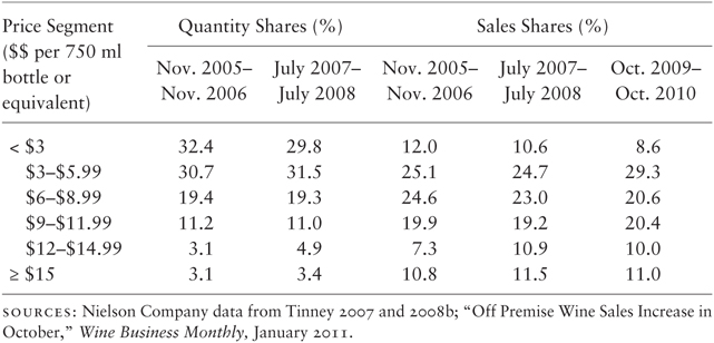
The thousands of wine products brought to the market each year vary in quality and are sold at a wide variety of prices. Because wine products range in price from $2.00 to more than $2,000 a bottle, the behavior of average price fails to tell the entire price story. Table 4 presents data on the market shares of wine products purchased from off-premises retailers for six different price segments for several time periods. Off-premises retailers, such as grocery and liquor stores, account for about 80 percent of the wine sold at retail establishments; the residual 20 percent is purchased primarily at restaurants and bars. Price is measured as dollars per 750 ml bottle or equivalent. Wine products priced below $3 a bottle are usually referred to as value or jug wines. Most of these are generic wines without varietal labels sold in containers larger than 750 ml. Wines in the $3 to $6 range are often called “fighting varietals.” These are low-priced varietal wines, such as Chardonnay and Merlot, made from grapes grown in high-yield vineyards, often from the Central Valley of California. Producers of these wine products attempt to mimic higher-priced varietal wines by using modern winemaking techniques, such as oak alternatives. Wine products priced above $6 are typically considered premium wines. This segment spans a relatively large range of prices from lower- to higher-end premium products. At the top of the price point scale are the luxury wines. These wines are typically made from low-yield, high-quality grapes, often from a single vineyard, and employ relatively high cost winemaking techniques like oak barrel maturation.
Columns 2 and 3 of table 4 report market shares by wine quantity for six price segments for two one-year periods: November 2005– November 2006 and July 2007–July 2008. The quantity of wine purchased falls at higher price points. For example, the fighting varietals priced between $3 and $6 account for about 30 percent of the off-premises market; the mid-priced $6 to $9 premium wines have about 19 percent of the market; the high-end premium and luxury wines priced above $15 have a relatively small market share of around 3 percent. During this three-year period, premium and luxury wines priced above $12 gained market share, while the market share of value wines below $3 declined. This phenomenon of substituting higher-priced wines for lower-priced wines is called “trading-up” in the wine industry. It is interesting to note that trading-up occurred even though real disposable income was falling, suggesting the possibility of a shift in tastes and preferences toward higher-quality wine products during this period. Columns 4 through 6 report market shares based on the dollar value of sales. Like quantity, fighting varietals also have the largest market share of sales accounting for almost 30 percent of off-premise wine expenditures in the most recent period. Sales shares tend to fall at higher price points with the exception of wines priced below $3.00. While these value wines account for about 30 percent of the quantity of wine sold, they generate less than 10 percent of the dollar value of sales. The sales-share data suggest that trading down occurred during 2009–10 as consumers spent more on fighting varietals and less on higher-end premium and luxury wines. This trading-down behavior occurred during a period of severe economic downturn with high unemployment and falling housing prices.
TABLE 4MARKET SHARE BY PRICE SEGMENT
Types of Wine Products Consumed
The five largest selling varietal wines in the United States are Chardonnay, Cabernet Sauvignon, Merlot, Pinot grigio/gris, and Pinot noir. Together they accounted for 51 percent of the dollar value of wine sales in off-premises retail stores between March 2011–12. Of these, Chardonnay and Cabernet Sauvignon are easily the two most important, with market shares of 21 and 15 percent respectively. To satisfy consumer tastes and preferences and generate adequate cash flow, the vast majority of wine firms include one or both of these in their product line. Consumers spend 13 percent more on red wine than white wine, and eight times more on varietal than generic wine. Imported wine accounts for 28 percent of retail store wine sales, with Italian wine the most popular (8.5 percent) followed by Australian (7.5 percent), Argentinian (2.5 percent), Chilean (2.4 percent), and French (2.3 percent).4
FACTORS AFFECTING WINE CONSUMPTION
The economic theory of consumer choice presented in chapter 1 implies that the amount of wine a typical individual is willing and able to purchase depends upon the price of wine, income, prices of goods related to wine, and tastes and preferences. The remainder of this chapter provides a detailed discussion of these factors and summarizes results from empirical studies that attempt to quantify and test their effects on wine consumption.
The Price of Wine
The price of wine is an important factor affecting wine consumption. The relationship between the quantity demanded and price of wine is illustrated graphically by a demand curve, such as the one in figure 1 in chapter 1, and represents either an individual’s demand for wine or the aggregate demand of all consumers collectively in a wine market. The negative slope of the demand curve reflects the law of demand. This is the commonsense notion that at lower prices, people want to buy more wine, and at higher prices, less, if other factors affecting wine demand such as tastes and preferences, income, prices of related goods, and wine quality remain unchanged. It also follows logically from rational decision making and the law of diminishing marginal utility. This section focuses on demand curves that aggregate over consumers. An aggregate demand curve exists for a single wine, such as Kendall-Jackson Chardonnay, or for a collection of wine products. The collection can be a particular wine brand composed of multiple products, red-wine products, white-wine products, varietal products, imported wine products, and other possibilities. Each of these can be viewed as a market demand curve for a different segment of the wine market. The highest level of aggregation is a demand curve for the entire wine market encompassing all wine products. It should be noted that at levels of aggregation above a single wine product, the notion of a demand curve becomes less precise, because it represents a collection of differentiated products, and the market price is an average of the product prices.
A common argument is that wine is different from a typical good or service, and that many individuals therefore violate the law of demand when making consumption decisions. Some individuals fail to respond to price changes because of brand loyalty and habitual behavior. Others, often referred to as wine snobs, derive more utility from the prestige a wine confers than from the enjoyment they get from actually drinking it. A prestigious wine is valued primarily because it is scarce and drunk by relatively few consumers. An increase in supply that reduces price and increases availability lowers the prestige value of the wine, and a wine snob will therefore buy less at the lower price. Alternatively, a higher price that reflects greater scarcity and lower consumption by others induces a wine snob to buy more. There are also other individuals in addition to wine snobs who engage in conspicuous wine consumption. These derive utility from the impression a wine makes on others about their economic or social standing. Because the price of a wine product conveys their socioeconomic status, the utility they derive from it depends on both its sensory characteristics and the price they pay for it. A higher price may induce these people to buy more, and a lower price, less. Finally, several studies suggest that many wine consumers use price to assess the quality of a wine. As a result, it is possible that some of these consumers will be induced to buy more at a higher price, and less at a lower price, even if the inherent quality of the wine, as reflected by its sensory characteristics, is unchanged.
The law of demand may be observed for a collection of consumers in a wine market even if this market includes individuals who are brand-loyal, wine snobs, habitual consumers, conspicuous consumers, or equate price with quality. First, consider the case of a market with unresponsive consumers. For example, suppose the market for Turning Leaf Chardonnay has a core of brand-loyal and habitual consumers, many of whom drink a glass each evening with dinner. It also has a fringe of consumers without these traits. If Gallo lowers its price, these core consumers may choose not to purchase more; however, some individuals currently drinking other wines or alcoholic beverages may enter the Turning Leaf market and buy this wine. In like manner, if Gallo raises its price, many habitual, loyal Turning Leaf drinkers may maintain their current consumption, but those fringe consumers who are less enthusiastic about this brand, or wine in general, may exit the Turning Leaf market and purchase a substitute wine, or beer, or spirits. At the market level, therefore, the law of demand may be largely a manifestation of new wine consumers entering as price falls and the less loyal consumers exiting as price rises.
As a second possibility, consider the market for a luxury wine like Screaming Eagle. Suppose some consumers in this market behave as wine snobs and others do not. If price falls, existing non-snobs may be inclined to consume more, new non-snobs will enter the market, and total consumption will rise. Increased consumption reduces the prestige value of Screaming Eagle for wine snobs, so some will leave the market. As they exit total consumption falls. However, the negative snob effect on total consumption must be smaller than the positive non-snob effect, and the market demand curve for Screaming Eagle will therefore be downward-sloping. If not, a reduction in price would result in a decrease in total consumption, which would increase prestige and induce wine snobs to purchase more.
Lastly, consider a wine market with conspicuous consumers or individuals who judge wine quality solely on the basis of price. If a sufficiently large number of these consumers exist in the market, then the aggregate demand curve for the wine or collection of wines may be upward-sloping. In this case, consumption would rise as price rises, at least up to some point. While theoretically possible, this violation of the law of demand seems unlikely, with the possible exception of a few very high-end luxury wines.5
Surveys of wine consumers and empirical studies of the wine market provide evidence in support of the law of demand. A 2006 survey by the Wine Market Council reported that more than 20 percent of wine consumers would drink wine more often at a lower price. More than 30 percent would consume more wine in restaurants if prices were reduced. Empirical studies consistently find that the demand curve for individual wines, different segments of the wine market, and the entire wine market slope downward. The following section discusses some of the findings of these empirical studies and their implications.
Empirical Studies
Empirical studies of the effect of price on wine consumption typically address three questions. First, does price have an effect on the amount of wine consumed? If it does, this is necessary but not sufficient evidence in support of the law of demand. Second, what is the direction of the effect? Does wine consumption rise or fall at higher prices? Verification of the law of demand requires evidence of a negative relationship between price and consumption. Third, what is the size of the effect? How responsive are consumers to a price change? Do consumers respond by altering their wine consumption by a relatively small or large amount?
To isolate the effect of price on wine consumption and draw valid conclusions, empirical studies use statistical methods to account for confounding factors, reverse causation, and chance. Failure to account for these potential problems, if they exist, may invalidate the conclusions of a study. A confounding factor is a variable that affects wine consumption and is correlated with wine price. For example, income is likely to influence the quantity of wine consumed. Suppose consumers with higher incomes tend to live in locations with higher wine prices than those with lower incomes. If income is not statistically controlled, then the estimate of the effect of price on wine consumption may also include the effect of income. Because these two effects are “confounded,” it is difficult to draw conclusions about the impact of wine price alone. Reverse causation occurs if price affects wine consumption and wine consumption affects price. Failure to control for the latter effect will result in a biased estimate of the effect of price on wine consumption, since this estimate will capture both the direct and reverse effects. At the market level, reverse causation is always a potential problem, because price and quantity consumed are determined simultaneously by the interaction of market demand and supply. Lastly, the effect of price on wine consumption observed in a sample of wine consumers may be either a real effect or a fluke that results from chance. To account for chance, most studies report a statistic called a p-value. The p-value is the probability that the observed effect is due to chance. For example, if the estimate of the effect of price on wine consumption has a p-value of 0.10, this indicates a 10 percent likelihood that the effect observed in the sample is the result of chance, and a 90 percent likelihood that it is a real effect. The smaller the p-value, the stronger the evidence that an observed effect is real and not a fluke.
To measure the size of the effect of price on wine consumption, most economic studies use the concept of price elasticity of demand. This is defined as the ratio of the percentage change in quantity of wine demanded to the percentage change in price. Because the changes in wine consumption and price are percentages, it is a unit-free measure of size. The estimate of price elasticity will be the same regardless of whether wine consumption is measured in gallons, bottles, cases, or any other meaningful unit. Moreover, a direct comparison can be made between the magnitudes of elasticity estimates of different wine products, wine and beer, wine and spirits, or wine and any other good or service, and determine for which good price has the biggest effect on consumers’ buying decisions. An elasticity of one serves as a useful benchmark. If the absolute value of price elasticity of wine is greater (less) than one, and the proportional change in consumption is therefore greater (less) than the proportional change in price, the demand for wine is elastic (inelastic) and consumers’ buying decisions are relatively responsive (unresponsive) to price changes. If the proportional change in the quantity consumed is equal to the proportional change in price, demand is unit-elastic and equal to one.
More than one hundred studies have analyzed the aggregate demand for alcoholic beverages in a wide variety of countries. These studies focus on the national market for wine, beer, and spirits. Wine consumption is typically measured as the quantity consumed per capita and encompasses the thousands of differentiated wine products purchased by consumers. An index of wine prices is used to measure the average price of wine. Together, these studies provide strong evidence in support of the law of demand for the aggregate consumption of alcoholic beverages in general and wine in particular. For the United States, studies report a wide range of price-elasticity estimates for wine, with an average estimate of −0.55. This indicates that a 10 percent reduction in the average price of wine products would increase consumption by 5.5 percent. The comparable estimates for beer and spirits are −0.52 and −0.60.6 These estimates suggest that consumers’ buying decisions are least responsive to changes in the price of beer and most sensitive for spirits. U.S. consumers tend to be somewhat more responsive to wine prices than consumers in other countries. The average elasticity estimate for eighteen other wine-consuming nations is −0.48.
The most important determinant of price elasticity is availability of close substitute products. If consumers can easily substitute another desirable beverage for wine—possibly beer, spirits, soda, or bottled water—then an increase in the price of wine will provide an incentive for them to switch and consume more of this other beverage in its place. The elasticity estimates suggest that for a typical consumer, beer has fewer desirable substitutes than wine, and spirits more. Another potentially important determinant of elasticity is the amount of time consumers have to adjust to a price change. Many may be in the habit of consuming wine, possibly as part of their lifestyles. A sharp rise in wine prices may have relatively little effect on their wine consumption in the short run. However, over time, they may decide to sample other beverages, such as beer and spirits, and eventually develop a taste for them. As a result, the longer these higher wine prices persist, the more willing they are to substitute other beverages for wine. Tsolakis, Riethmuller, and Watts (1983), a study using aggregate data for Australian wine consumers, estimated short-run and long-run price elasticities for wine in Australia and concluded that the demand for wine was inelastic in the short run, but elastic in the long run: the long-run elasticity estimate of −1.35 was more than three times as large as the short-run estimate of −0.43. The extent to which this behavior generalizes to U.S. wine consumers is unknown.
While a large number of studies have estimated the effect of price on wine consumption for the general U.S. wine market, relatively few have provided estimates for different segments of the market or individual wine products. A study by Stephen Cuellar and Ryan Huffman (2008) focuses on the off-premises retail segment and analyzes the behavior of consumers that purchase wine products from establishments such as grocery stores and wine shops. This excludes wine purchased at restaurants and bars, and directly from wine firms at tasting rooms, wine clubs, and over the Internet. In addition, they analyze consumer behavior in different segments of the off-premises market, including red, white, and varietal wines, as well as various price categories.
Cuellar and Huffman conclude that the demand for all types of off-premises retail wine products is elastic, with a price elasticity estimate of −1.23. This suggests that the demand for off-premises wine products is more elastic than overall wine demand, for which price elasticity is −0.55. We would expect consumers’ buying decisions to be more sensitive to changes in the prices of off-premises retail wine products, since there are more available close substitutes than for all wine products in general. If the prices of off-premises products increase, consumers can switch to products sold directly by wine firms and those available at restaurants and bars. To avoid an increase in the prices of all wine products, consumers would have to switch to beer, spirits, or nonalcoholic beverages, which many may view as poor substitutes.
Within the off-premises segment of the market, consumers are more responsive to changes in the prices of red wines than those of white wines. The demand for white wine is approximately unit elastic; the elasticity estimate for red wine is −1.23. Within each of these color segments, consumers are more price-responsive to changes in higher- than lower-priced red wines, but the opposite is true for white wines. A 10 percent increase in wine priced above $10 results in a 11.5 percent decrease in quantity demanded of reds; for whites, the quantity purchase falls by only 6.9 percent. For wine priced under $10, consumers are equally responsive to the prices of red and white wines, with an elasticity of about −1.10. One possible explanation is that consumers believe that there are fewer available close substitutes for higher-priced, higher-quality white wines than red wines. Alternatively, the average price of reds above $10 may be significantly higher than that of whites, and therefore absorb a larger fraction of consumer income. For example, suppose the average price of higher-end red wine is $40 per bottle, but only $25 for white wine. A 10 percent price increase in the former of $4 takes a larger fraction of income than a $2.50 increase in the latter. Because a given percentage increase in higher-priced whites results is a smaller income drain than reds, consumers are less sensitive to changes in white-wine prices.
Lastly, Cuellar and Huffman disaggregate the off-premises sector of the wine market into varietal segments and analyze the individual demands for six red and six white wines: Cabernet Sauvignon, Merlot, Pinot noir, Syrah, Zinfandel, Malbec, Chardonnay, Sauvignon blanc, Pinot grigio, Riesling, Chenin blanc, and White Zinfandel. All varietal products have downward-sloping demand curves, with estimated elasticities between −0.49 and −2.56. Once again this confirms the general applicability of the law of demand. Demand is elastic for ten of the twelve varietal products. Consumers are least responsive to price changes for Malbec and White Zinfandel, with elasticity estimates less than 1; they are most responsive for Chenin blanc and Riesling with estimates exceeding 2. Price elasticity of demand for the two most popular varietals, Chardonnay and Cabernet Sauvignon, are very similar. A 10 percent increase in price results in a 11 percent reduction in the quantity of Cabernet Sauvignon consumed and a somewhat larger 11.4 percent reduction in Chardonnay.
In another study, Cuellar, Lucey, and Ammen (2006) use data on off-premises retail sales to analyze the demand for a representative fighting varietal wine product: Gallo Turning Leaf Merlot. They report a price elasticity estimate of −5.7, indicating that a 10 percent increase in price will reduce quantity consumed by 57 percent. It is instructive to note that price elasticity for this individual red wine is more than five times larger than the elasticity for all reds priced at $10 or less. This is easily explained by availability of a large number of close substitutes. There are numerous substitutes for Turning Leaf Merlot in the low-price segment of the red wine market. These include Yellow Tail, Woodbridge, Bogel, Smoking Loon, Red Diamond, and Pepper Grove Merlot, as well as many more. Even a small increase in the price of Turning Leaf Merlot will induce large numbers of consumers to switch to a relatively less expensive substitute.
The Implications of Price-Elasticity Estimates
An important relationship exists between the price elasticity of demand for wine and consumer expenditures on wine. An understanding of this relationship is particularly useful for wine firms; consumers’ wine expenditures are wine firms’ sales receipts. If consumers’ buying decisions are quite responsive to a price change, and demand is thus elastic, a price reduction will result in an increase in consumer spending on wine and more revenue for wine firms. This is because the revenue loss from the lower price is more than offset by the revenue gain from proportionately more bottles sold. However, if demand is inelastic, a reduction in price will result in a decrease in consumer spending and wine-firm revenue. In this case, when consumers’ buying decisions are not very sensitive to a price change, the revenue gain from selling relatively few additional bottles is more than offset by the revenue loss from the lower price per bottle. On the other hand, if the price increases, expenditures and revenue fall when demand is elastic and rise when demand is inelastic.7
Cuellar and Huffman (2008) estimate that the price elasticity of demand for all types of off-premises retail wine products is −1.23. This implies that a 10 percent decrease in the price of wines sold in grocery and liquor stores will result in a 12.3 percent increase in the number of bottles sold, and therefore an increase in wine-firm revenue. This is indeed true if wine firms can sell their products directly to consumers at the retail price. However, wine firms in the aggregate sell about 90 percent of their wine to distributors at the wholesale price. Distributors then resell this wine to retailers, who receive the retail price. The price elasticity of demand for a product that a wine firm distributes through the three-tier channel may differ from the elasticity for the same product when sold at the retail level. To see why this is, consider the following example. Suppose a wine firm sells a product at a wholesale price of $10. After distributor and retailer markups, this wine is sold in off-premises retail establishments at a price of $20. Now, suppose the wine firm reduces the wholesale price by $1 to $9, and as a result retailers lower the retail price by $1 to $19. The 10 percent reduction in wholesale price lowers the retail price by only 5 percent. Given the retail price elasticity of −1.23, consumers will respond to the 5 percent reduction in retail price by purchasing 6.15 percent more. As a result, the wholesale price elasticity is 0.615. Even though demand is elastic at the retail level, it is inelastic from the perspective of the wine firm. As a general rule, the retail elasticity will be an accurate measure of the firm-level elasticity only if the distributor and retail margin as a percentage of the retail price is invariant to changes in the wine firm’s wholesale price. If this margin increases when the wholesale price changes, as in this example, then the demand curve for wine at the firm level will be less elastic than at the retail level. The opposite will be true if the distributor and retail margin declines.
If the objective of a wine firm is to maximize profit and the demand for its wine is inelastic, it will be motivated to charge a higher price. By increasing price, it will generate more revenue, even though consumers purchase fewer bottles of wine. Because it has to produce less wine to satisfy the lower level of consumption, its production cost will fall at the same time as revenue rises. However, at higher prices, consumers typically become increasingly responsive to additional price hikes, and eventually demand will become elastic.8 At this point, further price increases reduce both revenue and cost, and profit will therefore rise only if the revenue loss is less than the reduction in cost. This suggests that a profit-maximizing wine firm will prefer to operate in the elastic portion of its demand curve. Cuellar and Huffman estimate that the demand for Malbec and White Zinfandel are inelastic. This implies that producers of these two varietal wines could generate greater profits by raising prices. However, most Malbec sold in the United States is imported from Argentina. It may be that Argentinian producers are pricing their products at less than the market would bear to gain a foothold in the U.S. market. Most White Zinfandel is sold at a price below $10 in a segment of the market where a number of producers offer similar White Zinfandel products. While the demand for White Zinfandel as a whole is inelastic, the demand for the product of each producer is likely highly elastic. Short of colluding to set price, wine firms in this competitive segment of the market have little incentive to raise prices, since by doing so they might lose large numbers of consumers of their products to competitors.
Finally, if U.S. consumers tend to adjust their wine purchases slowly in response to changes in wine prices, as Tsolakis, Riethmuller, and Watts (1983) found for Australian consumers, demand may be inelastic in the short run and elastic in the long run. This implies that a strategy of short-term price discounting by wine firms to stimulate sales during an economic downturn may actually reduce both revenue and profit. Revenue will rise only if these price reductions are allowed to persist for a sufficiently long period of time for consumers to adjust their wine consumption behavior.
Income
A second important factor affecting wine consumption is income. Income determines an individual’s ability to purchase wine products. Consumers with higher incomes are able to buy more and higher-quality wine products if they so choose. The manner in which wine-buying decisions respond to a change in income depends upon the nature of the wine and consumers’ preference for it; this determines whether an economist classifies it as a normal or inferior good.
To illustrate the distinction between a normal and an inferior good, and how a consumer may respond to a change in income, consider the following example. Suppose that over the course of a year, Joe Oenophile consumes a mix of commodity, premium, and luxury wine products. Now, assume that his income increases, and that as a result, he buys more premium and luxury wine. Economists call these types of wines normal goods: as Joe’s income rises, he is willing and able to buy more, and as his income falls, less. For a normal wine product, Joe’s demand curve shifts to the right when his income increases: at the prevailing price of wine, whatever it is, Joe wants to purchase more. When Joe’s income decreases, his demand curve shifts to the left, and he demands less at any given price. However, the responsiveness of Joe’s buying decisions may differ for different normal wine products. For example, suppose that prior to the rise in income, he purchased eight bottles of premium and two bottles of luxury wine per year. He enjoys both types of wine, but each is subject to the law of diminishing marginal utility: the more he consumes during the year, the less utility he derives from each additional bottle. Because he consumes only two bottles of the luxury wine, he gets a relatively large amount of satisfaction from the consumption of an additional bottle. Also, given its high quality, the marginal utility of the luxury wine declines slowly as his annual consumption increases. An additional bottle of the premium wine yields him less utility, since he already consumes eight bottles per year, and declines more quickly as the number of bottles purchased increases. Because of these differences in the marginal utility of the two products, after Joe’s income rises, he will purchase more additional bottles of the luxury wine than the premium wine.
Suppose that after his income rises, Joe responds by buying less commodity wine. Economists call this an inferior good. At a higher level of income, Joe is able to buy more but willing to buy less, and his demand therefore decreases. Conversely, when Joe’s income falls, he is able to buy less but willing to buy more and his demand increases. Why would having a greater ability to buy a good induce a consumer like Joe to purchase less? Suppose that before he experienced the increase in income, the bulk of his annual wine consumption, say twenty bottles, was low-priced commodity wine. He would have much preferred to consume more premium and luxury wine but could not afford to do so. With a higher level of income, he is now able to replace some of the lower-quality wine with wine of higher quality.
Because goods can be either normal or inferior, there does not exist a “law of demand” for the relationship between income and the quantity of wine consumed. An increase in income may result in either an increase or decrease in the demand for a wine depending upon whether consumers perceive it as normal or inferior. The concept of an inferior good provides one possible explanation of the much discussed phenomenon of “trading up” and “trading down” in the wine market. In periods of rapid income growth, such as the late 1990s and the period from 2002 to 2007, trading-up occurs as the demand for higher-end premium and luxury wines rises and the demand for lower-end premium and commodity wines falls. In periods of falling income, such as 2008–9, trading down occurs as consumers substitute lower-priced commodity and premium wines for those at higher price points. This suggests that many consumers view generic wines and “fighting varietals” as inferior goods. They are not inferior because their absolute level of quality is low, but only because consumers prefer to consume less when they have more money to spend and more when they have less to spend.
Empirical Studies and Implications
To measure the size of the effect of income on wine consumption, most economic studies use the concept of income elasticity of demand.9 The income elasticity of total wine demand has important implications for the wine industry. Long-term income growth of the economy potentially affects the total amount and composition of wine products consumed in the United States. Rising per capita income enables consumers to buy more and higher-quality wine. A total income elasticity close to zero would suggest either that there is little difference in wine consumption across the income distribution of consumers or that the vast majority of consumers respond to rising income by substituting higher- for lower-quality wine products, with little net effect on overall consumption. A relatively large positive income elasticity indicates that rising income lifts total wine consumption, as well as possibly altering the composition of products purchased. A total income elasticity of less than zero has several alternative interpretations. It may indicate that wine is an inferior good for a typical individual; as income rises, a preponderance of consumers switch to other alcoholic or nonalcoholic beverages, which now become increasingly affordable. However, a more plausible interpretation may be that as income rises, a typical consumer drinks less wine, but wine of higher quality.
A total income elasticity of demand of greater than one implies that consumers spend a rising proportion of their incomes on wine as the economy expands, and therefore that the wine industry may well prosper with economic growth in the long run. However, it also suggests that economic recessions may have a relatively large negative impact on wine sales and profits as consumers respond to lower incomes in periods of economic contraction by sharply cutting back on wine consumption. Alternatively, an income elasticity of less than one suggests that the wine industry is less affected by the business cycle, but may have poor prospects for future growth. Of course, it is possible that the effect of income growth or decline could be offset by changes in wine prices, prices of other goods, and consumer tastes and preferences. It should be kept in mind that most studies use statistical methods to control for these influences, and therefore measure the change in wine consumption that results from a change in income, holding other factors constant.
Of the twenty-three studies undertaken to estimate the income elasticity of total U.S. wine demand, only one concludes that wine is an inferior good with an income elasticity of −0.58. Twelve studies find evidence that the demand for wine is income-elastic; eleven produce income-inelastic estimates. The average elasticity estimate of all twenty-three studies is 1.30, suggesting that the demand for wine is income elastic and that in the aggregate, consumers’ wine-buying decisions are quite responsive to changes in income and the business cycle. This is considerably larger than the average income elasticity estimate for beer and spirits of 0.45 and 0.87 and of 0.84 for the wine consumption of fifteen other countries.10 An income-elastic total demand for wine seems at odds with the prior observation that over the past sixty years, per capita wine consumption has been largely impervious to economic recessions, falling in only two of the ten downturns when aggregate output and income declined. A possible explanation for this is that the reduction in consumption resulting from falling income was countervailed by lower wine prices and a trend toward a stronger preference for wine. For instance, per capita wine consumption fell in the recession of 1953–54, in a decade when wine consumption was flat, and again in 1990–91, during a period when wine consumption had been trending down for the prior five years. It may be that during these recessions, the decrease in consumption resulting from declining income was not offset, and that in the recession of 1990–91, it was reinforced by an ongoing shift in preferences away from wine. During the other ten recessions, wine consumption was either flat or increased. These downturns occurred during periods when per capita consumption was trending up, possibly in large part because of more favorable preferences for wine. Moreover, during the recession of 2007–09, wine prices fell dramatically in both nominal and real terms, and relative to other alcoholic beverages. This may have helped to stem the fall in wine consumption.
Estimates of income elasticity of demand for different segments of the U.S. wine market and individual wine products are scant. One of the few studies to produce such estimates is the one by Cuellar and Huffman (2008) discussed previously, which analyzed wine demand for a number of different segments of the off-premises retail wine market. Its estimated income elasticity of 1.51 for all off-premises wine products indicates that a 10 percent increase in income will result in a 15.1 percent increase in demand for wine sold in grocery stores and wine shops. Products in the red, white, and all but one varietal segments of the off-premises market are normal goods, but income-elasticity estimates vary widely in size.11 For example, the estimate for white wine products of 2.35 is more than two times larger than the 0.89 estimate for reds. This suggests that the demand for whites is much more sensitive to cyclical ups and downs in economic activity than that for reds. Estimates of different price segments suggest this difference is largely explained by a low income elasticity of demand for red wines priced below $10. Income-elasticity estimates for varietal products vary from −0.43 for Merlot to 4.99 for Pinot noir. However, most of the estimates for varietals, including the negative income-elasticity estimate for Merlot, identifying it as an inferior good, are imprecisely measured, so it is difficult to draw conclusions with an acceptable degree of confidence.
Cuellar, Lucey, and Ammen (2006) reports elasticity estimates for two individual wine products: Turning Leaf Merlot, a lower-priced fighting varietal wine, and Sterling Merlot, a higher-priced premium wine. The estimate of −3.57 indicates that Turning Leaf is an inferior good: a 10 percent increase in income will induce a 35.7 percent decrease in quantity consumed. However, Sterling Merlot is a normal good, with an income elasticity of 1.76, indicating that a 10 percent increase in income will result in a 17.6 percent rise in consumption.
The Prices of Goods Related to Wine
Related goods are products that tend to be consumed either together or in place of one another. If an individual is inclined to consume wine with another product, such as steak, then the two are called complementary goods or complements. On the other hand, if an individual is willing to replace the consumption of wine with another product, such as beer, then the two are substitute goods or substitutes.
The price of goods related to wine is an important factor affecting wine consumption. An increase in the price of a complementary good such as steak induces an individual to consume less steak and less wine. This is because he or she prefers to drink wine when eating steak and consumes less steak at the higher price. This increase in the price of a complementary good is illustrated by a leftward shift of the demand curve as demand for wine decreases. An increase in the price of a substitute good, such as beer, provides an economic incentive for an individual to drink less beer and more wine. This is because he or she enjoys both of these beverages and is willing to consume more wine at the relatively lower price. As a result, the demand curve shifts to the right, and demand for wine increases. The opposite will occur when the price of a complementary or substitute good falls.
When analyzing the demand for wine, it is important to understand that the particular goods an individual perceives as substitutes and complements for wine depend upon his or her subjective tastes and preferences and may differ for different consumers. At the market level, substitutes and complements are determined by consumers’ buying decisions in the aggregate and apply to an average or typical wine consumer in the market. A good example of this is the relationship between wine and food. A common practice of professional wine writers is to mandate a web of rules that define which wine goes with which food. Cabernet Sauvignon, it is said, can only be consumed with beef, never with fish. Chardonnay is permissible with fish, seafood, and poultry, with the exception of oily fish. And the list goes on. These rules would seem to suggest, for example, that red wine and beef are complements and red wine and fish are unrelated. From an economic perspective, this is true only if it is consistent with the choices made by an average consumer in the marketplace. If a carefully performed empirical study finds that the demand for red wine increases when the price of fish falls, all else being equal, an economist would conclude that red wine and fish are complementary goods, regardless of how appalling this may be to wine professionals. Some prominent members of the wine community have in fact argued that esoteric “wine rules” such as these have adversely affected consumers’ preferences and demand for wine. The late Robert Mondovi, wine proprietor extraordinaire, once stated that when inundated with all of these rules a typical consumer says, “to hell with it; give me a beer, a scotch, a cup of coffee.”12
Empirical Studies and Implications
To determine whether a particular good is related to wine, and if so the size of the effect of the price of the good on wine consumption, economic studies use the concept of cross-price elasticity of demand.13 Cross-price elasticity of demand provides important information to wine firms. If two wines sold by different firms have a positive cross-price elasticity, then consumers view them as substitutes, and they therefore compete in the marketplace. The larger the cross-price elasticity, the greater the competition. If the two wines have a low cross-price elasticity, a firm has a greater ability to raise its price without losing many customers to its competitor. Conversely, a high-cross price elasticity informs a firm that even a relatively small price increase will induce a large number of its customers to switch to the other firm’s wine. Cross-price elasticity of demand, therefore, provides valuable information to a wine firm about the market in which it sells its wine and is a valuable tool in making pricing decisions.
Relatively few studies have been performed to estimate cross-price elasticities between wine and other products. Most of these focus on the total demand for wine, beer, and spirits, and use data on countries other than the United States. The results of these studies are mixed; some conclude that beer and spirits are a substitute for wine; others find evidence of a complementary relationship; still others suggest wine consumption is unrelated to that of beer or spirits. A study of U.S. consumers by Dale Heien and Greg Pompelli (1989) estimating cross-price elasticities for wine and other beverages found wine, beer, and spirits to be complementary, and wine, soft drinks, and juice to be substitutes. The sizes of the estimates are relatively small, suggesting that these beverages are weak complements and substitutes for wine. For example, the cross-price elasticity of wine and beer is −0.21. This implies that a 10 percent decrease in the price of beer results in a 2.1 percent increase in wine consumption. The estimate for wine and soda of 0.02 indicates that a 10 percent decrease in the price of soda will decrease wine consumption by a mere 0.2 percent. Heien and Pompelli conclude that the complementary relationship between wine, beer, and spirits can be explained by the effect of a change in the prices of these beverages on consumer real income. To elaborate, suppose that during the course of a month, Joe Oenophile consumes a certain amount of wine and beer. Given his preferences, he views wine and beer as beverages that can be consumed in place of each other. Assume that the price of beer decreases. Beer is now relatively less expensive than wine, so Joe is willing to drink more beer and less wine. However, the reduction in the price of beer gives Joe the ability to buy more of both beverages. This is because the purchasing power of his monthly income is higher, since he now pays a lower price for the beer he consumes. Assuming that beer and wine are normal goods, he is willing to buy more of each. If the income effect of the fall in the price of beer on Joe’s buying decisions is greater than the price effect that makes wine relatively more expensive, he will purchase more wine and beer, even though he does not prefer to consume the two together.
A study by Steven Buccola and Loren VanderZanden (1997) analyzed the demand for wine sold in retail stores in Portland, Oregon. Wine products were aggregated into four separate groups according to the region where the wines were produced: Oregon reds, California reds, Oregon whites, and California whites.14 The researchers were interested in whether a typical consumer in Portland views these types of wine products as substitutes or complements, and how strongly they are related. They conclude that Oregon and California reds are substitutes, and Oregon and California whites are substitutes. The demand for Oregon wines is highly sensitive to a change in the price of California wines. A 10 percent reduction in the price of California reds (whites) decreases the consumption of Oregon reds (whites) by 19.8 (11.9) percent. However, the demand for California wines is much less responsive to a change in the price of Oregon wines. A 10 decrease in the price of Oregon reds (whites) reduces the consumption of California reds (whites) by a much smaller 3.7 (6.5) percent. This suggests that if California wine firms lower prices in the Portland market by say 10 percent, a large number of Portlanders will quickly switch to these wines, and Oregon producers will lose significant market share. To prevent these consumers from switching to California wines, Oregon wine firms would have to respond by reducing the prices of their reds by 53 percent and their whites 18 percent. Conversely, if California producers increase prices, Oregon wine firms can gain substantial market share by keeping their prices constant, because many Portlanders will switch to the relatively lower-priced Oregon Pinot noir, Chardonnay, and Pinot gris to avoid paying relatively higher prices for California wines. Buccola and VanderZanden also find evidence that a typical Portlander views red and white wines as complements. When the price of red wine falls, the consumption of white wine increases. The same is true of red wine consumption when the price of white wine decreases. One possible explanation is that a typical Portlander consumes both red and white wines. The particular wine selected depends upon how well it pairs with the food consumed at a meal.
Cuellar, Lucey, and Ammen (2006) estimates the cross-price elasticity of demand for three Merlots in the fighting varietal segment of the market, Turning Leaf, Woodbridge, and Sutter Home. While all three pairs of these wines have large positive cross-price elasticity estimates, the closest substitutes are Turning Leaf and Woodbridge, with an estimate of 5.76. These estimates provide empirical evidence of the highly competitive nature of the market for fighting varietal wines.
Tastes and Preferences for Wine
The economic theory of consumer choice implies that tastes and preferences are potentially an important factor affecting wine consumption. A favorable change in consumers’ preferences for wine will result in an increase in demand and shift the demand curve to the right. An unfavorable alteration in tastes will have the opposite effect. Unfortunately, economic theory provides little guidance on what factors determine tastes and preferences, and why these factors might change. There is no economic theory of preference determination. Economists recognize that individuals’ preferences differ and can change over time. However, economic theory typically assumes that preferences are stable during the period of time under consideration. The theory is then used to predict how consumers will respond to changes in prices and income. This permits the economist to attribute a change in consumption to a change in preferences only after a careful consideration of other factors. Playing by these rules minimizes the temptation to rely too heavily on the amorphous notion of tastes to explain changes in consumption. When performing empirical studies of consumer behavior, most economists attempt to account for tastes and preferences either by assuming they are an unobservable random variable or by including variables they believe may be correlated with preferences. This section begins by discussing a number of factors that economists and wine professionals speculate may influence consumers’ tastes and preferences for wine. It then discusses the findings of some empirical studies that have attempted to analyze patterns and changes in wine consumption associated with tastes and preferences.
Copious factors may affect consumers’ preferences for wine. Most of these fall under one of four general categories: demographic characteristics, knowledge and information, cultural influences, and health considerations. Demographic characteristics include variables such as age, education, gender, race, marital status, occupation, family size and composition, and geographic location. The argument is that these sorts of personal characteristics and social factors help to shape tastes for wine and may explain wine consumption patterns independent of prices and income.
Preferences may also be influenced by wine knowledge and available information. One source of information about wine is advertising. There is an ongoing debate in economics about whether advertising is primarily persuasive or informational. Advertising that provides consumers with information about wine characteristics and prices may reduce their cost of obtaining this information when making buying decisions without altering preferences. Advertising designed to persuade consumers to drink a particular wine product or wine in general may change preferences and shift the wine demand curve. Some industry observers have argued that much of the downward trend in per capita wine consumption that occurred from 1986 to 1995 can be explained by a decrease in wine industry advertising that caused a shift in consumers’ preferences towards other beverages. In 1991, the wine industry spent $92 million on advertising. By 1995, this had fallen to $60 million in inflation-adjusted dollars. During this same year, Anheuser-Bush devoted $577 million to advertising its beer products, while Coors spent $205 million. Pepsico spent $1.3 billion on advertising soda, more than twenty times as much as the entire wine industry. Dairy, pork, and egg producers have successfully increased the demand for their products by undertaking industrywide advertising campaigns with slogans like “Got milk?” “the other white meat,” and “the incredible edible egg.”15
Much attention has also been given to the role of wine critics in shaping the preferences of consumers. Most critics use the 100-point rating scale instituted by Robert Parker in the 1980s to evaluate the quality of thousands of different wine products. Some wine professionals maintain that critics’ scores provide valuable information to consumers without influencing their preferences. Given the thousands of different wine on the market, consumers cannot typically taste a wine to evaluate its characteristics before making a purchase. As a result, wine critics’ scores provide consumers with useful information. Most of their advocates acknowledge that wine scores depend largely upon the subjective tastes of critics, and different critics often assign different scores to the same wine. However, they maintain that consumers learn which critics have preferences similar to their own, and that if they purchase a highly scored wine that does not agree with their taste, they will not buy another bottle. Like the advertising controversy, other wine professionals argue that consumers’ preferences are significantly influenced by critics’ scores. They contend that many consumers believe that these scores are a better measure of wine quality than their own preferences. Critics, through their scores, essentially teach consumers to enjoy certain wine styles, and by doing so reshape consumers’ preferences to match their own tastes. Regardless of whether wine critics’ scores affect or reflect consumer’s preferences, almost all agree that they have a significant effect on wine demand and the wine industry. Producers, distributors, and retailers use these numbers as an important marketing tool. Many consumers buy wines based on the scores they receive from critics, which are often posted in retail stores and provided on restaurant wine lists. Many retailers report that products receiving a score of 90 points or above are in great demand and sell out quickly; those with a score below 90 quite often suffer the opposite fate. It is argued that wine scores also affect the types of products wine firms produce. The bold, intensely flavored, fruit-forward style favored by a majority of wine firms today is often attributed to Robert Parker, who has a strong preference for this style and rewards wine products that possess these sensory characteristics with high scores.
Wine preferences may also be influenced by a consumer’s level of wine education. Many consumers perceive wine as a complex product. Those who are less educated and informed about the intricacies of wine and how it pairs with food may be inclined to purchase less or prefer other beverages, such as beer or spirits, that are less confusing and intimidating. Many argue that the wine industry fostered a mysterious, formal, and elitist image of wine for years, which had a negative effect on demand. However, more recently this has changed, since consumers have become more educated about wine. Knowledgeable consumers, it is argued, have a more favorable preference for wine, leading to increased demand.
Cultural heritage and social tradition have long been recognized as factors influencing wine preferences. In many European nations, drinking wine with meals is a venerable tradition. If more consumers in the United States incorporated this routine into their lifestyles, the resulting shift in preferences would likely have a large impact on wine demand. Popular culture may also influence the taste for wine. After the hit movie Sideways disparaged Merlot and extolled Pinot noir, sales of Merlot slowed and Pinot noir rose, particularly for wines costing $20 per bottle or more (it had a relatively small negative effect on the consumption of Merlot priced below $10 per bottle).16
In the past, the Wine Market Council, a leading trade organization for the wine industry, has argued that the most important factor affecting wine consumption is consumers’ perception of wine’s health effects. This conclusion has been supported by Wine Market Council research and anecdotal evidence. In 1991, for example, the widely watched television news show 60 Minutes aired a segment on the so-called French paradox, looking into why the French have a much lower incidence of heart disease than Americans, even though they consume a high-fat diet, many smoke, and relatively few exercise. Medical research suggested that this might be the result of regular French consumption of red wine, 60 Minutes asserted, and the show summarized a growing body of evidence of the positive health effects of moderate alcohol consumption. Within the next couple of months, U.S. red wine sales increased by 30 percent.17 As additional medical studies were published on the positive health effects of wine, demand continued to grow. Many wine industry professionals maintain that a shift in preferences resulting from the perception of wine as a healthful beverage has been a key factor in the inexorable growth of per capita U.S. wine consumption since the early 1990s.
Empirical Studies
Most empirical studies that analyze the effect of factors related to tastes and preferences on wine consumption focus on consumers’ demographic characteristics. As stated previously, surveys indicate that a majority of U.S. wine drinkers are highly educated, middle-aged, married professionals. However, this may not necessarily reflect preferences for wine. Individuals with these characteristics also tend to have higher incomes than others. When drawing conclusions about the effect of demographic characteristics on wine demand, empirical studies attempt to control for income and other potential confounding variables. This is necessary to isolate the independent effect of various demographic factors on wine demand that may be related to wine preferences.
The empirical findings for age, marital status, and occupation are consistent with the descriptive characteristics of wine drinkers. Controlling for other factors, married individuals consume more wine than those who are single, widowed, or divorced; the middle-aged consume more wine than those who are younger and older; and professionals consume more wine than non-professionals. The results for education are mixed and inconclusive. This may suggest that individuals with more education tend to consume more wine because of their higher incomes, rather than having a stronger preference for wine than those with less education. These studies also find evidence of greater than average wine consumption by urban white Californians knowledgeable about wine with few or no children.18
Wine Quality
The final important factor affecting wine consumption is wine quality. If it is assumed that a rational individual prefers higher-quality to lower-quality wine, the maximum amount he or she is willing to pay for a given quantity of wine will increase with quality. Equivalently, at a given price, the amount of wine purchased will increase with quality. As a result, higher wine quality increases demand and shifts the demand curve to the right; lower wine quality has the opposite effect. Economists have developed a theoretical framework that can be used to analyze and measure quality and its effect on wine demand and prices. This is the topic of chapter 12.