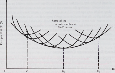
■ Definition: The long-run average cost (LAC) curve shows the least cost of production for each output level when all inputs may be varied. It is a hypothetical construct, composed of pieces of many different SAC curves. It is the locus of points on the various SAC curves which allow each output level to be produced at lowest cost, given the ability to change plant size (or vary the input of capital).
To derive the long-run average cost curve we can proceed by finding the SAC curve that relates to every level of fixed factors. Each level of capital (fixed factor) input will give rise to a TP curve, from which we ca n deri ve a TVC curve and ultimately obtain the appropriate SAC curve as we did above. This procedure would give us a series of SAC curves, each with a slightly larger capital input level as we move from left to right. As shown in Figure 6-8, the long-run average cost (LAC) curve is the “envelope curve” of all these short-run curves. A corollary of this is that for any point on the LAC curve there is an SAC curve lying tangent at that point.
Note: The LAC curve may not be a smooth U-shaped line for every firm in the real world, since the smooth U-shape depends upon the availability of a large number of plant sizes, with the sizes of these plants varying by relatively small increments from the smallest available to the largest available. In many industries there are only a few alternative sizes of plant, each significantly different in size from the next largest and the next smallest.
Example: Consider the case of a small private airline company that plans to initiate a feeder service from a remote area to a major city. In choosing the aircraft for this route the firm must, in effect, choose its size of plant, since light aircraft are available in 4-, 6-, 8-, and 10-seat models. In this case, plant sizes are available only in discretely increasing, rather than continuously increasing, sizes, and the LAC curve will exhibit a series of kinks, or scallops, rather than being a smooth line. In Figure 6-9 we show the LAC curve as the heavy line encompassing only those sections of each SAC curve which allow output to be produced at lowest cost.
LAC
Output Units (0
FIGURE 6-8. Long-Run Average Cost Curve: Envelope Curve of All Short-Run Average Cost Curves
FIGURE 6-9. Long-Run Average Costs with Discrete Plant Size Differences
The four SAC curves represent the available plant sizes, with the subscripts indicating the maximum number of seats in each plant size. Note that each SAC becomes vertical at the point where it reaches its maximum output (passenger) level. The LAC curve is the envelope curve of these four SAC curves; it contains kinks at points ,4, B, and C, where it becomes less costly (per passenger) to choose the next largest plant size.
Note that if there were an aircraft available that seated 5 passengers (including the pilot), the SAC curve of that plant size would have nestled between SAC 4 and SAC b , and it would have caused the kink in the LAC curve at point A to disappear. Similarly, if planes were also available with 7 and 9 seats, the other kinks might be removed or at least replaced by smaller kinks. With plant size continuously variable, the LAC curve would be a smooth line. In the real world, however, the LAC curve is most likely to exhibit kinks because plant size is not continuously variable.
Choice of Plant Size in the Long Run. In the short run the firm is confined to the plant size it is currently operating, but in the long run it will be able to either enlarge or reduce its plant to the size that best serves its objectives. Thus, if a firm finds itself with a plant that is either too large or too small in relation to its current quantity demanded, it may undertake the steps necessary to reduce or increase plant size. If it wants to reduce plant size, it has to find buyers for plant and buildings, wait until employment and other contracts expire, and so on. If the firm wishes to increase its plant size, it may need to order the fabrication and construction of new plant and buildings, search for new managers, hire and train more workers, and so on. All these things are possible; they simply take time to accomplish.
Given the freedom to choose any size of plant in the long run, which one should the firm choose? It should choose the plant size that minimizes the average cost of producing the firm’s desired output level. Refer back to Figure 6-8 and suppose that the firm wishes to produce output level Q, (because Q { is the net-worth-maximizing output level, for example). Three different plant sizes that can produce output level Q , are shown in Figure 6-8, but the plant size chosen will be the one that produces this output level at the lowest average cost. Note that the plant size chosen will be the one with its SAC curve just tangent to the LAC curve at the desired output level. For “kinky” LAC curves, as shown in Figure 6-9, the plant size chosen will be the one with its SAC curve coextensive with the LAC at the desired output level. For example, when quantity demanded is expected to be 8 passengers (including the pilot), the optimal plant size is the 10-seat aircraft.
In many cases the costs are known, but demand is uncertain. How then does the firm select its plant size? We can apply expected value analysis to find the plant size that minimizes the expected value of average costs. Since the uncertain demand may be represented by a probability distribution of potential demand outcomes, we can transfer those probabilities to the output levels necessary to satisfy each of those demand levels, and note that each output level has a known average cost level in any particular plant. This process is demonstrated in Table 6-3. The probability distribu-
Table captionTABLE 6 3. The Expected Value of Average Costs: Choice of Plant Size When Costs Are Known but Demand Is Uncertain
QUANTITY DEMANDED | PLANT A | PLANT B | |||
Potential | Prob- | Average | Expected | Average | Expected |
Outcome | ability | Cost | Value | Cost | Value |
11 ] | [2] | [3] | [4] = [2] X [3] | [5] | [6] = [2] X [5] |
500 | 0.05 | 3.00 | 0.15 | 5.00 | 0.25 |
1.000 | 0.15 | 2.50 | 0.375 | 3.00 | 0.45 |
1,500 | 0.25 | 2.00 | 0.50 | 1.75 | 0.4375 |
2,000 | 0.35 | 2.75 | 0.9625 | 1.50 | 0.525 |
2,500 | 0.15 | 3.50 | 0.525 | 2.00 | 0.30 |
3,000 | 0.05 | 4.50 | 0.225 | 3.00 | 0.15 |
Expected Values | 2.7375 | 2.1125 |
tion of quantity demanded is shown in the first two columns. The average cost at each of those output levels in a particular plant (plant A) is shown in column 3, and the expected value of average cost in that plant is calculated in column 4, where each value is the product of the value in column 3 multiplied by the probability of its occurring, from column 2. The expected value of average cost in an alternate plant (plant B) is calculated in columns 5 and 6.
Note that plant A has lower average costs for smaller output levels but higher average costs for the larger output levels. Further inspection shows that where the weights (demand probabilities) are highest, plant B has the lower average costs. Thus we see that the weighted average costs, or the expected values of average costs, are lower (at $2.1125 per unit) in plant B. Assuming that these are the best two plant sizes available, the firm should install plant B based on this expected demand situation. 8
Note: A totally erroneous procedure would be first to calculate the expected value of quantity demanded (in this case 1,775 units) and then to base one’s decision on the average cost level at that expected value of output in each plant. A quick interpolation between the average cost figures at 1,500 and 2,000 units in Table 6-3 will confirm that this procedure would give an underestimate of average costs in both cases, since larger and smaller outputs tend to have higher costs per unit.
'though the initial costs of plant B are probably higher than plant A, this difference is already incorporated into the analysis, since we are dealing with average costs. The fixed costs per unit include deprecation, which is an expense charged against revenues in each period to reflect the cost of the plant and equipment during the period. Also included would be any additional costs resulting from the larger size of p ant B, such as additional salaries and maintenance expenses. Thus total cost per period is expected to be lower in plant B at the expected quantity demanded. In the following chapter wesha^l express some miseiv mgs about the way that depreciation is typically calculated, since it involves an allocation of thTnomfnal cost over a number of periods and may not accurately reflect the “economic" cost of the plant. Furthermore the depreciation expense is deducted in nominal, rather than present-value, terms.
The firm’s choice of its plant size to minimize the average cost (or expected value of the average cost) of production typically leads the firm to build a plant with production capacity greater than the level (or expected value) of quantity demanded. This excess capacity is evident in both the examples referred to previously (in Figures 6-8 and 6-9). In both cases the plant selected has the capacity to produce at a rate substantially higher than the (expected value of) quantity demanded. How do we measure excess capacity? In an absolute sense, the firm can continue to increase output until the SAC curve becomes vertical, but by the time that happens the marginal cost will be approaching infinity. Thus the absolute capacity is not a very useful reference point from which to measure excess capacity.
■ Definition: The full capacity of a plant is usually referred to as the output level at which MC begins to rise above SAC. Although additional output could be produced by adding more units of the variable factors, MC would typically rise very steeply. Firms usually avoid such “overfull capacity” production wherever possible, preferring instead to produce at slightly less than full capacity so that they have in reserve some excess capacity that can be utilized if the firm’s demand increases. When the market is growing, excess capacity buys the firm some time, allowing it to serve an expanding market without unit costs rising prohibitively (or at all) while it is in the process of building a larger plant. Excess capacity also allows a firm to produce at a rate higher than its current demand rate, to rebuild depleted inventories, to recover from a labor strike or mechanical breakdown, or to take advantage of a competitor’s problem. Thus we measure excess capacity as the difference between the firm’s current output level and the output level at which MC rises above SAC, and we recognize that after excess capacity is all used up the firm still has some overfull capacity it may wish to utilize, if it is profitable to do so.