In this chapter we review the “theory of the firm,” which is a series of models that attempt to explain and predict the price and output decisiom of^the firm. These models, which bring together the demand analysis of Chapters 3 and 4 with the cost analysis of Chapter 6, are usually covered in introductory and intermediate microeconomics courses. However, this chapter should not prove too difficult for a student who has not had these courses, since it brings together material from earlier chapters that is familiar by now. If you have taken microeconomics courses previously, this chapter will provide more than a simple review, because it takes a somewhat novel approach
and introduces some more recent concepts.
The first thing to learn about the theory of the firm is that there is no single model of the firm’s behavior. In fact, there are literally dozens of models of the firm, each one designed to explain or predict a firm’s behavior in a particular market situation. Each model of the firm consists of four structural assumptions, which define the demand and cost conditions facing the firm, and three behavioral assumptions, which define how the firm is expected to behave in its market situation as it pursues its
objective.
Traditional price theory delineates four basic market forms, namely, pure competition, monopolistic competition, oligopoly, and monopoly. Pure competition consists of many firms producing identical products in an environment of full information—all firms know where to buy the cheapest inputs, and all consumers know where to buy the cheapest products. Firms operating in pure competition are called price takers, because the price of their product is determined by the market forces of demand and supply. Excess demand for the product will drive the market price up, and excess supply will drive the market price down. Since all firms are selling exactly the same piod- uct and consumers have full information about all firms’ prices, a firm will sell noth-
ing if it raises its price above the market price. Conversely, the firm has no incentive to reduce its price below the market price, since it is small relative to the size of the market and can sell all that it wants to at the market price.
The other three market forms are characterized by product differentiation, and the state of information is not complete. In fact, lack of information may be one of the bases for consumers’ differentiating between the products of rival suppliers. Monopolistic competition consists of many firms with slightly differentiated products. Oligopoly consists of a relatively small number of firms whose products are typically substantially differentiated from each others’ through some combination of product design, promotional efforts, and place of sale. 1 Monopoly consists of a single seller of a product that has no close substitutes; thus the product is highly differentiated from the products of all other firms.
Firms operating in monopolistic competition, oligopoly, and monopoly are called price makers^ because they can adjust the price of their product up or down in order to pursue their objectives. The firm’s ability to set prices derives from the differentiation of its product. Each firm can raise its price to some extent without losing all its customers, since the remaining customers believe that the product is worth the extra price being asked.
In Table 9-1 we show the four traditional market forms in terms of the underlying structural and behavioral assumptions. Note that the essential differences between the four market forms arise from assumptions 1 and 4. Thus it is the number of firms and whether or not the firms’ products are differentiated that essentially characterize the firms into the four traditional market forms. The three types of price-maker markets are each characterized by differentiated products. Assumption 7 also differs across the market types, but note that this difference is related to assumption 1. When there are many firms in the market, each firm can safely expect no reactions from rivals following the adjustment of its strategic variable, since the effects of this adjustment are spread over many rivals, making an insignificant impact on each one. Conversely, in an oligopoly, where there are relatively few rivals, the firm should expect its strategic actions to have a noticeable impact on the sales of each of its rivals, and therefore expect them to retaliate in some situations. Monopolists expect no reactions because there are no rivals in their markets.
In managerial economics we are concerned with the firm’s pricing problem— namely, to set its price at the level that will best serve its objective. Consequently, we
'A" oligopoly could, in theory, have undifferentiated products. In practice a “pure oligopoly” is hard
the anrihute f h Pr t ^ “ *7 3,1 attnbUteS ° f the prod -t are identical acres" firmsTus not only the attributes of the firms core product, such as steel, but all other (peripheral) attributes of the product'
including the convenience of purchasing, the delivery schedules, the product warrantyandtheTnterpep sonal relationship between the purchasing agent and the salesperson, must be equal across all firms Even if
e'ntTr P /nm C ,S ""I 11 ' tHe Sa 7’ 7 S Unlikdy th3t ,he buye >' wi » find one seller a little more conve think th P eaS , ant t0 buy from ' The ex »stence of imperfect information may make the buyer
think there is a difference between the sellers even if there is not. If the buyer has any preference for one
cerned 0 ^ PnCeS ^ eqUa '’ the " ^ products are differentiated as far as the buyer is con-
TABLE 9-1. Market Forms and the Seven Assumptions Underlying Them
PRICE
TAKERS PRICE MAKERS
Pure Monopolistic
Competition Competition Oligopoly Monopoly
Structural assumptions:
1. Number of sellers
2. Cost conditions
3. Number of buyers
4. Demand conditions
Many Many Few One
Underlying the number of sellers is an assumption concerning barriers to entry. The absence of barriers to the entry of new firms means that there will be many firms in the market. Substantial barriers to entry in oligopoly markets limit the rivals to a few. Insurmountable barriers to entry allow the monopolist to remain the only seller of its product.
For all models we can assume diminishing returns in production in the short run, causing MC to rise. This is not important in oligopoly and monopoly, where constant or declining MC may prevail.
For all models we assume many buyers, so that the dominant force in the pricing decision will not be one, or a few, strong buyers. Variants of the oligopoly and monopoly models, known as oligopsony and monopsony, cover the strong-buyer situation.
Identical Very similar Close No
substitutes substitutes substitutes substitutes
Behavioral assumptions:
5. Objective function For all models we initially assume short-run profit maximization.
This may be inappropriate for oligopoly, where time horizons typically extend beyond the short run, since high short-run profits may induce the entry of new competitors to cause a more competitive market for the firms later in the planning period.
6. Strategic variable In all models we assume the firm can adjust price and quantity sup¬
plied, although once the price is in equilibrium, pure competitors will adjust only their quantity supplied. Firms in the other three market types may also adjust their promotional efforts, product design, and distribution channels.
7. Expectation of rivals’ reactions
None, since there are many firms in both these market types. Firms are all small relative to their market, so their actions will go unnoticed by rivals.
Rivals may ignore or match the firm’s actions, depending on what serves their
objectives.
None, since there are no close substitutes for the monopolist’s product.
are more concerned with the price-making models than with the price-taker model of pure competition. Nevertheless, the firm may face conditions approaching pure competition in some situations, so a quick review of the pure competition model is appropriate.
In pure competition the equilibrium price is determined by the interaction of the market forces of supply and demand. There are many buyers and many sellers, each too small relative to the market to influence directly the general price level. In aggregate, however, their demand and supply decisions lead to the determination of the equilibrium market price. The market demand curve is negatively sloping, and the market supply curve is positively sloping, as shown in the left-hand part of Figure 9-1. If, at a particular price level, such as P u supply exceeds demand, there will be downward pressure on prices, because of the desire of firms to reduce inventories to preferred levels. Each firm reduces price in order to clear its excess inventories and thus avoid costs associated with holding those excess inventories. Since many firms will be independently reducing their prices, the market price falls. One firm alone reducing its price would not cause a reduction in the general price level, since it could sell all it wishes at the lower price without any competing firm suffering a significant loss of sales, because of the assumption that firms are small relative to the market. But the combined effect of many firms reducing their prices causes a significant loss of sales to those competitors that have not reduced their prices. This in turn causes those firms to suffer excess inventory, and they too will be motivated to reduce price.
Thus excess market supply leads to a reduction in the market price. The lower price causes an increase in the quantity demanded and at the same time causes the
Price
The market
Price
One representative firm*
*Note that the output scale is much smaller for the firm than for the market.
FIGURE 9-1. Price and Output Determination in Pure Competition
firm to be willing to supply a somewhat reduced amount. Prices will continue to fall until finally supply equals demand, as shown in Figure 9-1.
Conversely, if there is excess demand at a particular price level, such as at P 2 in Figure 9-1, there will be upward pressure on prices, because of the willingness of some buyers to pay more than the market price rather than go without the product. Firms will find they can raise their price slightly yet still sell all they wish to produce, since although other firms may be maintaining their price at P 2 , those firms are unable to supply all the buyers willing to purchase at price P 2 , and some of the remaining buyers are willing to pay more than P 2 to obtain the product. The firms setting price P 2 then see that they too can ask for a higher price, and the combined effect is for the market price to move upward. As it does, the quantity demanded is reduced as some buyers drop out of the market, and the quantity that suppliers are willing to put on sale increases, until finally supply equals demand and no further incentive exists to raise prices. The price P* in Figure 9-1 is thus the equilibrium price and is determined not by the actions of any one firm but by the combined effects of individual firms’ actions.
Given the market price, the purely competitive firm must decide what output level to produce in order to maximize its profits. Profits are maximized when the difference between total revenues and total costs is greatest. Since the firm is small relative to its market, it can sell all it wants to at the market price, and its demand curve is therefore a horizontal line at the market price level, as shown in the right-hand part of Figure 9-1. Since the price is constant regardless of the number of units sold, marginal revenue is equal to price, and the demand and marginal revenue curves are coextensive. The short-run average cost (SAC) and marginal cost (MC) curves are added to the firm’s graph, and we note that MC = mr at output level q*. To maximize its profit the firm chooses the output level q*, where marginal cost rises to equal marginal revenue. Producing one more unit of output would cost more than the revenue it would generate (MC > mr), and producing fewer units of output would save less cost than the revenue forgone (MC < mr). The firms profit can be visualized as the rectangle P*ABC , since profit is the product of the price-cost margin (P* — C) times the output level Oq*. 2
Note: Do purely competitive markets exist? There are certainly some markets that have many buyers and many sellers. The most difficult condition to find is that of identical products. All buyers must regard all products from the competing suppliers as identical in all respects. Buyers cannot have personal preferences for particular sellers, nor have differing expectations of quality or after-sales service, nor find it more
or less convenient to buy from one seller rather than from another. The package of attributes constituting the product must be viewed as identical in all respects.
Example: Perhaps the only market in which this condition is fulfilled is the stock exchange, at which hundreds of buyers and sellers meet anonymously (through an agent) to buy and sell a company’s stock. Each share in the company has the same rights, benefits, and obligations attached (for each class of shares), and no buyer is likely to care about the identity of the previous owner. In fact, the theory of finance is based on the pure competition model.
Applications of the purely competitive model as an explanatory or predictive device will be inappropriate to the extent that the seven assumptions involved do not accord with the reality of the situation being explained or predicted. The major value of the purely competitive model is probably as a pedagogical model. It allows the theory of the firm to be introduced in a relatively simple context, free of the complications introduced by product differentiation and fewness of buyers or sellers. It thus forms a basis upon which we can build an understanding of more complex theories of the pricing behavior of firms.
Monopolists and monopolistic competitors can safely ignore the reactions of their rivals, in the former case because there are no close rivals, and in the latter case because the firms are each small relative to the market and are expected to have insignificant impact upon each others’ sales. Oligopolists may ignore the probable reactions of rivals, but they do so at their own risk. The sales and profits of oligopolists are interdependent, or “mutually dependent”—the competitive actions of one have a significant impact on the sales of the others and may provoke a competitive reaction. Recognition of mutual dependence (RMD) means that the firms recognize and take into account the probable reactions of rivals before undertaking a competitive strategy. We shall consider oligopoly pricing (with RMD) in the next section. We shall not consider “non- RMD” oligopoly pricing at all, because of the space constraints of this text and because of the topic has limited relevance to managerial economics. 3
'These “myopic” oligopoly pricing models, such as the Cournot and Edgeworth models, do have some pedagogical value, since they demonstrate quite forcefully the implications of myopia in oligopolistic markets. In short, failure to recognize mutual dependence leads to the downward progression of prices to a price floor, as in the Cournot model, or to the fluctuation of prices between a price floor and a price ceiling, as in the Edgeworth model. A particularly thorough treatment of these classical models of duopoly (two sellers) under conditions of unrecognized mutual dependence is found in A. Koutsoyiannis, Modern Microeconomics , 2nd ed. (London: Macmillan, Inc., 1979), pp. 216-33.
Monopolies exist when there is a single seller of a product in a particular market. They persist over time if the entry of new firms is prevented by barriers to entry. Barriers to entry are additional costs that a potential entrant must incur before gaining entry to a market. These costs may arise because the existing firm controls an essential raw ma-i) terial, the best location, necessary information, the right to produce the product (such as a “patent” or a government mandate), and so on. Consumer loyalty to the existing firm poses a barrier to a potential entrant, since the new firm would have to spend substantial amounts on advertising to offset it. In some cases the entry cost is infinite (where it is impossible to acquire the necessary input or permission to produce), and in other cases the cost is simply high enough to prevent a potential entrant from making a profit in the foreseeable future.
Some monopolies are natural monopolies , in the sense that the market would inevitably be served by a monopoly even if some other market form were to exist initially. This situation occurs when the monopolist’s output capacity is large relative to the market demand. In terms of the long-run average cost (LAC) curve and the monopolist’s demand curve, the quantity demanded at the monopolist’s price would occur where the LAC curve is still falling. Thus a single firm will benefit from economies of plant size by expanding to supply the entire quantity demanded. If an oligopoly initially existed, the firms would have a profit incentive to merge with (or take over) each other to form a monopoly and subsequently benefit from the economies of plant size.
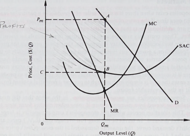
The profit-maximizing monopolist will wish to expand output until marginal costs rise to equal marginal revenues. Since this firm faces the entire market demand, the firm’s demand curve and the market demand curve are one and the same. Thus the market marginal revenue curve is the firm's marginal revenue curve. We saw in Chapter 4 that the marginal revenue curve associated with a negatively sloping linear demand curve has the same vertical intercept on the graph and twice the slope of the demand curve. In Figure 9-2 we show the market demand curve (D) faced by the monopolist and the corresponding marginal revenue (MR) curve. Superimposed on these are the cost curves of the monopolist—the short-run average cost (SAC) and marginal cost (MC) curves. The profit-maximizing monopolist produces up to the point where marginal costs per unit rise to meet the falling marginal revenues. This point occurs at output level Q m . Notice that every unit to the right of Q,„ has a marginal cost greater than its marginal Revenue; it therefore will not be produced. Conversely, every unit to the left of Q m costs less than it earns (marginally or incrementally); it therefore vv/// be produced and sold. The firm’s profits can be visualized as the rectangle P„, ABC ih Figure 9-2.
Note: Monopolists in the real world usually do have some peripheral competition from distant and partial substitutes. The post office experiences competition from the telephone company and from such delivery services as United Parcel Service (UPS) for some of the services it provides. The electricity company competes with the gas com-
FIGURE 9-2. Price and Output Determination for a Monopoly
pany in some households. Bootleggers compete with the liquor control board in some areas. In all these cases, however, the extent of substitution of these products for the monopolist’s product is quite small. Thus the cross elasticity of demand between the monopolist’s product and the distant substitutes, over the market as a whole, is quite low.
In monopolistic competition markets the firm must choose price knowing that the consumer has many close substitutes to choose from. If the price is too high, in view of the consumer’s perception of the value of the differentiating features of the firm’s product, the consumer will purchase a competing firm’s product instead. Thus the monopolistic competitor must expect a relatively^lastic demand response to changes in its price level. Yet at the same time, it expects to be able to change price without causing any other firm to retaliate and, consequently, without causing a change in the general price level in the market. This is possible because the firm is one of many firms, and it expects the impact of its actions to be spread imperceptibly over all the other firms, giving no one firm any sufficient reason to react to the initial firm’s price change.
Monopolistic competition is so called because it has elements of both monopoly and pure competition. The firm has a significant amount of the monopolist’s pricing power by virtue of the differentiation of its product. It can change price up and down
without experiencing the extreme response of pure competition. For price increases it will suffer a loss of sales, but this loss is not total, as it would be for the pure competitor. Like a monopoly, the monopolistic competitor can adjust the price upward or downward to the level which maximizes its profits. But like the pure competitor, the monopolistic competitor has many rivals in the short run, compounded by the free entry of new firms in the long run.
Example: Monopolistically competitive markets are found where a large number of vendors gather to sell similar products to a gathering of potential buyers. The weekly fruit and vegetable market in some communities may be characterized as monopolistic competition. Similarly, the gatherings of artisans selling souvenirs and other goods in tourist resorts act like monopolistic competitors. 4
The situation of a representative firm in monopolistic competition is depicted in Figure 9-3. Since the demand curve is negatively sloping, the marginal revenue curve must lie below the demand curve, having twice the slope and the same intercept point. The monopolistically competitive firm maximizes its profits at the price and output level where marginal revenue equals marginal costs. Thus price will be set at P i and quantity at Qp, profits are shown as the area P\ABC.
The prices set by monopolistic competitors need not be at the same level. In real- world situations we should expect to find slight price differentials between and among monopolistic competitors, with some firms being able to command slightly higher prices or larger market shares because of the market’s perception of greater value in the product of some firms as compared with others. Firms with more convenient locations, longer operating hours, and quick service, for example, can obtain a premium for what is otherwise the same product (e.g., brand A bread). Quality differences inherent in the product will also form the basis for price differences. 5
“'Be wary about characterizing markets as monopolistically competitive unless there are many firms in a relatively compact area and consumers could reasonably be expected to consider purchasing from any one of the firms. Note that seller location (or convenience of purchase) is a relevant attribute in the purchase decision for most consumers. Several industries have a large number of producers but are not characterized by monopolistic competition, since the markets for these industries are sparsely dispersed across the nation. There may be thousands of fast-food outlets in North America, but each one seldom competes with more than half a dozen other sellers in its local market. Similarly, there are hundreds of gas stations in and around a large city, but each one is in competition with the three or four gas stations nearest to it, rather than with every other gas station in the entire city. This spatial aspect of some industries means that, rather than being monopolistically competitive, their markets are characterized by intersecting oligopolies, -with each firm competing directly with only a few nearby rivals.
Trice and market share differences arise in the asymmetric monopolistic competition model, where both cost and product differentiation are allowed to differ among firms. This is a considerably more complex model that the symmetric case outlined above, in which it is implicit that the "representative firm has the same cost structure and product differentiation advantages as all other firms. The asymmetric model will not be considered here except to note that it allows greater realism, at the expense of greater complexity, by explicitly considering differing cost and product differentiation situations between and among firms.
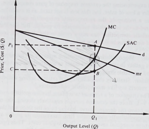
FIGURE 9-3. Price and Output Determination for a Representative Firm in Monopolistic Competition
9.3
Definition: Oligopolies are markets in which there are only a few sellers (The word oligopoly is derived from the Greek word oligos, meaning few and the Latin word pohs meaning seller.) Recall that we use the word few to mean a number small enough
so that the actions of any one firm have a noticeable impact on the demand for each of the other firms.
Example: In the real world the great majority of market situations are oligopolies Prominent examples are the automobile, steel, aluminum, and chemical industries!
hese are national and, in some cases, international oligopolies. In your local or regional area, you will notice many more oligopolies. There are probably only half a dozen new car dealerships from which you would consider buying a new automobile
area' and T* ^ Y 3 ^ Se ' lerS “ 3 multitude of °*her lines of business in your area, and these qualify as oligopolies if the actions of any one seller have a significant impact on the sales of any other seller.
Oligopolists are mutually dependent because there are only a few of them sharing a part.cular market. and an, one firm’s sales gain, resulting from a pdce redue tion for example, will be accompanied by sales losses for its rivals. The rival firms must be expected to react to their loss of sales, probably by also reducing price in order
to win back their lost customers. The oligopolist that ignores its mutual dependence will thus receive a rude shock when sales volume and profits do not turn out the way they were expected to. Moreover, such myopic price cutting could precipitate a “price war” which could inflict heavy financial losses on all firms. Conversely, a price increase that is ignored by rivals may lead to a substantial loss of market share and profitability, since at least some of its customers will switch to a rival firm’s product.
Thus the oligopolist should attempt to predict the probable reaction of rivals to its strategic actions, and decide whether or not an action is likely to be worthwhile in the final analysis, before taking that action. The firm’s expectation of its rivals’ reactions is known as its conjectural variation. The firm’s conjectural variation may be defined as the expected percentage change in the rivals’ strategic variable (such as price) over the contemplated percentage change in the firm’s strategic variable. Thus conjectural variation will be zero when the firm expects rivals to do nothing in reaction to its action, unity if the firm expects rivals to exactly match its action, and more than ^(or less than) unity if rivals are expected to adjust their strategic variables by a greater (or lesser) percentage.
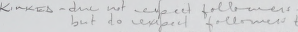
When oligopolists do recognize their mutual dependence, there are a variety of different conjectural variations they might make. We shall first examine the kinked demand curve model. b This model assumes that the firm’s conjectural variation will be twofold: for price increases the firm expects no reaction from rivals, since the other firms will be content to sit back and receive extra customers who switch away from the firm raising its price; and for price reductions the firm expects rivals to exactly match the price reduction in order to maintain their shares of the market.
Since the firm’s conjectural variation for price increases is zero, it envisages a ceteris paribus demand curve at all prices above the current level, this curve being more or less '-elasthA depending primarily upon the degree of substitutability between its product and rival products. In contemplating price reductions, however, the firm envisages a different kind of demand curve, known as a mutatis mutandis demand curve, meaning that it takes into account all reactions induced by or concurrent with the firm’s price adjustment. In this case the mutatis mutandis section of the demand curve represents a constant share of the total market for the product in question, because if all firms move their prices up or down in unison, their relative prices will remain the same, and we therefore expect each of them to maintain its market share. 7
This model was initially proposed separately by R. L. Hall and C. J. Hitch, “Price Theory and Business Behavior,” Oxford Economic Papers , May 1939, pp. 12-45; and by P. M. Sweezy, “Demand under Conditions of Oligopoly,” Journal of Political Economy, August 1939, pp. 568-73.
7 Note that while the ceteris paribus demand curve is appropriate for “independent action” by a firm not expecting reactions, the mutatis mutandis demand curve is appropriate for “joint action by firms, taking into account rivals’ reactions.
In Figure 9-4 we show a firm’s current price and output levels as P and Q. For prices above P, the firm envisages the relatively elastic ceteris paribus demand curve shown by the line dv4. For prices below P, it envisages the relatively inelastic mutatis mutandis demand curve shown by the line A D. The demand curve facing the firm is therefore dv4D, being kinked at the current price level. The marginal revenue curve appropriate to this demand curve will have two separate sections. The upper section, shown as dB in Figure 9-4, relates to the ceteris paribus section of the demand curve and therefore shares the same intercept and has twice the slope of the line dA. The lower section, CMR, relates to the mutatis mutandis section of the demand curve and is positioned such that it has twice the slope of the line A D, and if extended up to the price axis would share its intercept point with the line A D similarly extended.
You will note that there is a vertical discontinuity in the marginal revenue curve, shown as the gap BC in Figure 9-4. Given the foregoing, it is apparent that the length of this gap depends upon the relative slopes of the ceteris paribus and mutatis mutandis demand curves, 8 which in turn are related to the elasticity of demand under the two conjectural variation situations. If the firm is a profit maximizer, its marginal cost curve will pass through the gap BC. If P and Q are the profit-maximizing price and
'^2_oF : f' r
M(0_> IM C*
MR
Output Level (Q)
—rW
c,tu«-£
MC
FIGURE 9-4. The Kinked Demand Curve Model of Oligopoly
8 See G. J. Stigler, “The Kinky Oligopoly Demand Curve Economy, 55 (October 1947).
and Rigid Prices,” Journal of Political
output levels, this relationship implies that outputs to the jeft j >f Q would have marginal revenues exceeding marginal costs, while outputs to the right^of Q would have mar ginal costs exceeding marginal revenues. This observation is true only if the MC curve passes through either of the points B or C or through some point in between. 9 The oligopolist’s profits are shown by the rectangle PAEF in Figure 9-4.
Price Rigidity in the Kinked-Demand-Curve Model. The KDC model is not a complete theory of price determination, because it is unable to tell us how the firm arrives at the initial price and output levels. Given this starting point, however, the model is able to tell us several things that are important to our understanding of oligopoly mar- ketsv^First) it offers an explanation of the observed rigidity of oligopoly prices in the face of changing cost and demand conditions. Recall that in each of the models of firm behavior we have examined so far, the firms set price where marginal costs equal marginal revenue. If either costs or demand conditions change, one of these marginal curves shifts, and a new price level is required if the firm is to maximize profits under the new conditions. In the KDC case, however, the marginal cost and marginal revenue curves may shift to a considerable degree without a new price level becoming appropriate, as we shall see.
In the KDC model the firm does not wish to change price as long as the marginal cost curve passes through the gap in the marginal revenue curve. Thus costs could increase so that the MC curve moves upward until it passes through point B in Figure 9-5 without the present price becoming inappropriate. Conversely, if variable costs fall, the MC curve could sink downward until it passes through point C, and price P would remain the profit-maximizing price. As long as marginal revenue exceeds marginal costs for higher prices and is less than marginal costs for lower prices, the present price remains the optimal price. Of course, profits are smaller when costs are higher, but profits are(maximized when the MC curve passes through the MR gap^
Now consider changes in the demand situation. In most real-world market situations, quantity demanded at the prevailing price level fluctuates up and down over time as the result of seasonal, cyclical, or random influences on the factors determining demand. But as we show in Figure 9-6, demand at price P could fluctuate over the range Q to Q’ without causing the MC curve to pass outside the relevant MR gap. At quantity Q, the MR curve is shown by d^CMR, and the MC curve passes through point C. This is the extreme leftward point to which the demand curves could shift and yet still allow the MC curve to pass through the gap. The extreme rightward shift of demand, which allows P to remain as the profit-maximizing price, is found when the MC curve passes through point B’, as it does at output Q '. Thus demand could fluctuate over the relatively wide range Q to Q ' at price P without the firm wishing to change its price. Profits are lower when demand is lower, but are maximized at price P
’See D. S. Smith and W. C. Neale, “The Geometry of Kinky Oligopoly: Marginal Cost, the Gap, and Price Behavior,” Southern Economic Journal, 37 (January 1971), pp. 276-82.
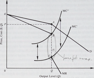
FIGURE 9-5. Price Rigidity in Oligopoly despite Changing Cost Levels
'MR'
FIGURE 9-6. Price Rigidity in Oligopoly despite Changing Demand Levels
as long as the demand shift is not so large as to cause the MC curve to miss the gap in the appropriate MR curve. 10
Price Adjustments in the Kinked-Demand-Curve Model. Let us look briefly at a cost change that will tbad to a change in price. As implied previously, if the change is such that the new MC curve no longer passes through the MR gap, the firm will want to change price. In Figure 9-7, we show a shift of the marginal cost curve from MC to MC', causing it to intersect the MR curve at point B '. The initial price P is no longer the profit-maximizing price, since marginal cost exceeds marginal revenue for all the output units between Q' and Q. The new profit-maximizing price is thus P', where the MC' curve intersects the MR curve. The firm therefore raises its price to P' and experiences a reduction in its quantity demand from Q to Q '.
FIGURE 9-7.
l0 George Stigler (see footnote 8), and Julius Simon. “A Further Test of the Kinky Oligopoly Demand Curve,” American Economic Review , December 1969, each presented empirical findings to indicate that prices in oligopolies were adjusted more frequently than were prices in monopoly markets, thus appearing to refute the KDC model’s prediction that oligopoly prices would be adjusted less frequently than would monopoly prices. Jack Hirshleifer, in his Price Theory and Applications , 2nd ed. (Englewood Cliffs, N.J.: Prentice-Hall, Inc., 1980), p. 400, points out that there are reasons to expect monopoly prices to be adjusted relatively infrequently, such as fear of attracting regulatory scrutiny and management’s pursuit of their own objectives, and these reasons may have been stronger for the monopolists than was the KDC effect for the oligopolists. In addition, it should be recognized that the KDC model is just one model of oligopoly. Other models, such as the price leadership models and the conscious parallelism variant of the KDC model, explain how price adjustments are facilitated in oligopoly. Thus we should recognize that the KDC model does not purport to describe the conjectural variations of all oligopolists at all times. But for those firms at those times when the split conjectural variation is appropriate, it is a valuable addition to the decision maker’s toolbox.
Notice that the firm raised its price independently, with the expectation that no other firm would follow its price increase; consequently, it lost part of its market share. Since the firms price-output coordinate is now point A ', it must envisage the new mutatis mutandis demand curve, A'D', for any contemplated price reduction. Thus the firm’s share-of-the-market demand curve has effectively shifted to the left as a result of its independent price increase. But the firm, being a profit maximizer by assumption, would rather increase profits than worry about market share, and hence it prefers the higher profit situation at price P ', given the cost increase that upset the initial equilibrium situation.
Alternatively, we could show the demand curves shifting to the right to such an extent that the firm prefers to raise price (and lose part of its market share) in order to maximize profits. Conversely, we could show the marginal cost curve failing sufficiently or the demand situation declining sufficiently, causing the MC curve to cut the lower section of the marginal revenue curve. In either of these two cases, the firm would cut its price, notwithstanding its expectation that rivals would immediately follow suit, because cutting price allows profits to be maximized. Since all rivals match the price reduction, all firms maintain their market shares at the lower price level.
Thus the KDC model predicts that firms will hold price steady, despite the fluctuations of variable costs or demand over a significant range of cost or output levels. Outsi de the limits set by the requirement that the MC curve pass through the gap in the MR curve, the firm will be motivated to change price. It will raise or lower price to the new profit-maximizing level, whether or not it expects rivals to do likewise.
Under some conditions the firm’s conjecture that other firms will ignore its price increase may give way to the expectation that other firms will follow a price increase rather than ignore it. Such a situation may arise when a cost increase applies to all firms, such as an increase in the basic wage rate or an increase in the cost of an important raw material. In the case of cost increases that apply to all firms, the individual firm may reasonably expect that all firms would like to maintain profit margins by passing the cost on to consumers. Especially if there is a history of this practice in the industry, the firm’s conjectural variation for a price increase, up to the extent necessary to pass on the cost increase, may be unity.
■ Definition: The simultaneous adjustment of prices with the expectation that rivals will do likewise has been called conscious parallelism . 11 The firms consciously act in a parallel manner, given their expectation that all other firms are motivated to act in the same way.
"See W. Hamburger, “Conscious Parallelism and the Kinked Oligopoly Demand Curve,” American Economic Review , 57 (May 1967), pp. 266-68.
The relevant demand curve for a consciously parallel price increase is the muta- tis mutandis demand curve. As indicated in Figure 9-8, the kink in the demand curve moves up the mutatis mutandis section to the new price level chosen. It will kink at the level that passes on the cost increase, because the firm expects that any further price increase will not be matched by rivals and therefore expects to experience a more elastic demand response above that price level. The firm’s conjectural variation is unity up to the price level that is expected to be agreeable to all firms, and it is zero for price levels above that. 12
In terms of Figure 9-8, the firm has experienced a shift in its marginal cost curve from MC to MC'. Based on its expectation that rival firms have suffered a similar cost increase and will be raising their prices, the firm raises its price from P to P’ in order to pass on the cost increase to consumers. The firm expects its price-quantity coordinate to move from point A to A ', along the mutatis mutandis , or share-of-the-mar- ket, demand curve. If its expectation (that rivals will similarly raise prices) is borne out, it will in fact move to A ', its new kinked demand curve will be d' A'D, and its new marginal revenue curve will be d'5'C'MR.
FIGURE 9-8. Conscious Parallelism in the Kinked-Demand-Curve Model of Oligopoly
l2 The extent to which price is raised depends on the extent to which the firm expects other firms to raise prices simultaneously; it may be more than, less than, or equal to the cost increase. It would be (joint) profit maximizing to raise price ail the way to the point where the MC curve cuts the mutatis mutandis MR curve (extended upward). But if some firms are not expected to raise price that far, the demand curve will kink and that MR is thus inappropriate.
Since all firms are expected to act jointly, each firm expects to maintain its share of the market at the higher price level, and, by passing on the cost increase to consumers, each firm expects to maintain its profit margin per unit (the difference between price and average costs). In the next chapter we see that the prevalent practice of markup pricing allows firms to practice conscious parallelism in the real world, even when they don’t know how their demand curves slope away from the present price level.
A number of oligopoly models rely upon the notion of price leadership to explain the upward adjustment of prices in oligopoly markets. The major difference between conscious parallelism and price leadership is that in the former situation all firms take the initiative in adjusting prices, confident that their rivals will do likewise, whereas in the latter situation one firm will lead the way and will be followed within a relatively short period by all or most of the other firms adjusting their prices to a similar degree. The price leader is the firm willing to take the risk of being the first to adjust price, but, as we shall see, this firm usually has good reason to expect that the other firms will follow suit. The risk involved here relates especially to price increases, since if the firm raises price and is not followed by other firms, it will experience an elastic demand response and a significant loss of profits before it can readjust its price to the original level.
Note: Conjectural variation for the price leader isjunity^kince this firm expects all rivals to adjust prices up or down to the same degree that it does. For the price followers, conjectural variation is zero for self-initiated price increases, since price followers do not expect to have all firms follow their price increases. For price decreases, the price follower may expect all firms to follow suit to protect their market shares, and so the conjectural variation is unity for price reductions. It should be immediately apparent to the reader that the price follower faces a kinked demand curve.
There are three major types of price leaders: the barometric price leader, the low- cost price leader, and the dominant firm price leader.
The Barometric Price Leader. As the name implies, the barometric price leader possesses an ability to accurately predict when the climate is right for a price change. Following a generalized increase in labor or materials costs or a period of increased demand, the barometric firm judges that all firms are ready for a price change and takes the risk of sales losses by being the first to adjust its price. If the other firms trust that firm’s judgment of market conditions, they too will adjust prices to the extent indicated. If they feel the increase is too much, they may adjust prices to a lesser degree and the price leader may bring its price back to the level seemingly endorsed by the other firms. If the other firms fail to ratify the price change, the price leadership role could shift from firm to firm over time and will rest with the firm that has sound
knowledge of market supply and demand conditions, the ability to perceive a consensus among the firms, and the willingness to take the risk of sales losses if its judgment on these issues is faulty. 13
The Low-Cost Price Leader. The low-cost price leader is a firm that has a significant cost advantage over its rivals and inherits the role of price leader largely because of the other firms’ reluctance to incur the wrath of the lower-cost firm. In the event of a price war the other firms would suffer greater losses and be more prone to the risk of bankruptcy than would the lower-cost firm. Out of respect for this potential power of the lower-cost firm, the other firms tacitly agree to follow that firm’s price adjustments. 14
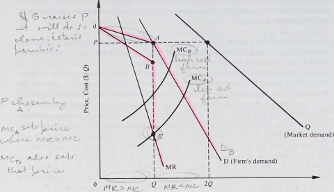
In Figure 9-9 we show the demand curve D as the curve faced by either firm when each firm sets price at the same level. This curve is thus a mutatis mutandis demand curve, predicated upon the simultaneous adjustment of the other firm’s price to the same level. In price leadership situations price adjustments are more or less concurrent, and the demand curve D in this case represents a constant (half) share of the total market at each price level. 15 The marginal cost curves of the two firms are shown as MC^ for firm A, the lower-cost firm, and MC fl for firm B, the higher-cost firm. The lower-cost firm maximizes its profit from its share of the market by setting price P and output level Q, and firm B follows the lead and also sets price P.
Given that it sets price P, what output level should the higher-cost firm produce? Being a profit-maximizing firm, by assumption, it will simply choose the output level that maximizes profits, subject to the (self-imposed) constraint that its price will be the same as the price leader’s. The demand curve facing firm B is the kinked line dAD. If the high-cost firm raises its price, it expects to do so alone, along the ceteris paribus section d A. If it sets its price below P, the other firm will match this price reduction to avoid having its sales fall dramatically. The marginal revenue curve associated with the kinked demand curve d A D is the disjointed line dBCMR. Firm B should therefore choose output level Q, since below this output level, marginal revenue exceeds marginal costs, and above this level, marginal costs exceed marginal revenue. The firms thus share the market equally at the price level chosen by the lower-cost firm.
1 ’Barometric price leadership was first proposed by J. W. Markham, “The Nature and Significance of Price Leadership/' American Economic Review, December 1951, pp. 891-905. For a thorough discussion of barometric price leadership, see F. M. Scherer, Industrial Market Structure and Economic Performance. , 2nd ed. (Chicago: Rand McNally & Company, 1980), chap. 6.
N This agreement is likely to be ruled illegal price fixing if the firms explicitly agree on price levels. Price fixing is discussed in Appendix 10A.
15 If product differentiation is symmetric, the share of the firms will be equal when prices are equal, and each firm would lose sales at the same rate following an independent price increase. This is a simplifying assumption, since in practice we should expect to find asymmetric product differentiation, whereby market shares are unequal when prices are equal, and the slopes of the firms’ ceteris paribus demand curves are not necessarily equal.
Output Level (g)
FIGURE 9-9. Low-Cost Firm Price Leadership: Simple Two-Firm, Identical Products Case
Price Leadership with Price Differentials. When product differentiation is asymmetric we should expect a range of prices among the rival firms, reflecting the different cost and demand situations facing each firm. Price leadership in this situation requires one slight modification to the preceding analysis. The price leader may adjust its price by a certain amount, and the price followers will adjust their prices by the same percentage as is represented by the price leader’s price adjustment. Thus the relative price differentials that prevailed prior to the price changes are unchanged, and no firm expects to gain or lose sales from or to a rival. The price leader simply initiates an upward (or downward) adjustment in the entire price structure of that particular market.
In Figure 9-10 we show a situation in which three firms produce asymmetrically differentiated products. Firm A is the acknowledged price leader and sets price P A , selling Q a units. Firms B and C are price followers, not wishing to initiate price adjustments in case this might precipitate a price war in which the lower-cost firm A would have a definite advantage. Firm B’s price is above the price leader’s price, and firm C’s price is below the other two prices. Firm B’s product may be a higher-quality item desired by a relatively small segment of the market. This firm’s higher cost level may well be the result of higher-quality inputs and more hand finishing of the product, for example. Firm C’s product is both lower priced and more expensive to produce, as compared with the price leader’s. The lower price may be due to the market’s percep-
V—4) t p,
371
Models of the Firm's Pricing Decision
\
\
\
(Price Leader)
Firm A
Firm B
(Price Follower No. I)
Firm C
(Price Follower No. 2)
U
CL.
o
0
—V \
\
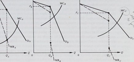
FIGURE 9-10. Low-Cost Firm Price Leadership: Two or More Firms, Asymmetric Product
Differentiation and Cost Conditions
tion of inferior after-sales service, an inferior location, or absence of other attributes, while the higher costs may be the result of more expensive sources of the inputs, inefficiencies in production, or a plant size too small in view of the present output level.
The price followers face the kinked demand curves shown because they expect no reaction from rivals for price increases but expect the price leader and the other price follower to match any price reductions. The price leader’s demand curve is simply the mutatis mutandis demand curve: The price leader expects the other firms to follow both price increases and price reductions. If, for example, the price leader’s costs increase, it will adjust price upward along the curve. The price followers, who have probably incurred a similar cost increase, will follow the lead and adjust prices upward. But for this particular price increase they do not expect ceteris paribus ; they expect that the other firms will be simultaneously adjusting their prices upward (or have seen them do so). Thus the kinks in the price followers’ demand curves will move upward, extending the mutatis mutandis section of their demand curves, as in the conscious parallelism case shown in Figure 9-8.
We shall see in Chapter 10 that the common business practice of markup pricing allows firms to adjust prices to cost increases by a similar proportion. We turn now ter the third type of price leader.
The Dominant-Firm Price Leader. As the name implies, the dominant firm is large relative to its rivals and its market. The smaller firms accept this firm’s price leadership perhaps simply because they are unwilling to risk being the first to change prices, or perhaps because they are afraid that the dominant firm could drive them out of
Pricing Analysis and Decisions
business, for example, by forcing raw-material suppliers to boycott a particular small firm on pain of losing the order of the larger firm. In such a situation the smaller firms accept the dominant firm’s choice of the price level, and they simply adjust output to maximize their profits. In this respect they are price takers, similar to pure competitors who can sell as much as they want to at the market price. Like pure competitors, they will want to sell up to the point where their marginal cost equals the price (equals marginal revenue). The dominant firm recognizes that the smaller firms will behave in this manner and that it must therefore choose price to maximize its profits with the knowledge that the smaller firms will sell as much as they want to at that price.
The first task of the dominant-firm price leader is, therefore, to ascertain how much the smaller firms will want to supply at each price level. Since each of the smaller firms will want to supply up to the point where MC = MR, and since MR = P in a situation where the individual firm is so small that it does not influence market price, each of the smaller firms will regard its MC curve as its supply curve. Note that a supply curve shows the quantity that will be supplied at each price level. At each price level the firms supply the amount for which marginal cost equals price. The MC curve therefore indicates how much the firm will supply at each price level. It follows that a horizontal aggregation of these curves will indicate the total amount that the smaller firms will supply at each price level. In Figure 9-11 we depict this aggregation of the smaller firms’ marginal cost curves as the line EMC S .
Knowing how much the smaller firms will supply at each price level, the dominant firm can subtract this quantity from the market demand to find how much demand is left over at each price level. This “residual” demand can be measured as the horizontal distance between the EMC 5 and the market demand curve D at each price
FIGURE 9-11
level, and is shown as the demand curve d R in Figure 9-11. Only at prices below P 0 is there any demand left for the dominariTfirm after the smaller firms have supplied their desired amounts. This residual demand curve is the amount that the dominant firm can be assured of selling at each price level, since the smaller firms will have sold as much as they wanted to and yet there remain buyers willing to purchase at those price levels.
The dominant firm will choose the price level in order to maximize its own profits from this residual demand. The marginal revenue curve associated with the residual demand curve is shown as the curve mr in Figure 9-11. The dominant firm’s marginal cost curve is depicted by MC D . The dominant firm therefore selects price P D and output <2 D in order to maximize its profits. Faced with the price P D , each of the smaller firms produces up to the point where its marginal costs equal that price, and hence the smaller firms in aggregate produce the output level <2,. Since the residual demand curve was constructed to reflect the horizontal distance between the EMC 5 and the D curves, the total amount supplied to the market, LQ, is equal to the market demand, and an equilibrium situation exists. The dominant firm thus chooses price to maximize its profits under the constraint that the smaller firms will supply the amount at that price level which will maximize their profits.
Note: An interesting long-run implication of the dominant-firm-price-leadership model is that if the chosen price allows the smaller firms to earn economic profits, the dominance of the large firm will be eroded over time. The reason for this erosion is that in the long run the small firms will expand their plant sizes in search of even greater profitability, and new firms will enter the industry—if the barriers to entry can be overcome—in search of this profitability. Unless the market grows faster than the small firms, the residual demand remaining for the dominant firm must be reduced, and the price leader will be forced to set a lower price and accept a reduced market share. Eventually, of course, the dominant firm will no longer be dominant, and the above system of market price determination will give way to some other form of price leadership, conscious parallelism, or independent price setting.
Example: Alcoa is said to be an example of a firm that was initially a monopoly, later a dominant-firm price leader, and more recently simply one of several large oligopolists in the aluminum industry. 16 Alcoa was effectively a monopoly at first because it held most of the known reserves of bauxite, from which aluminum is derived. As more bauxite was discovered, other firms entered the industry but were small in relation to Alcoa. As time passed and Alcoa’s chosen price level allowed the other firms to prosper and grow, Alcoa’s dominance in the industry waned to the point where it is no longer the price leader at all. Rather, Alcan has emerged as the low-cost price leader because of its cheaper source of electric power.
"’See J. V. Koch, Industrial Organization and Prices, 2nd ed. (Englewood Cliffs, N.J.: Prentice-Hall, Inc., 1980), pp. 282 and 289.
374 Pricing Analysis and Decisions