1. D
We need to use implicit differentiation to find 
![]() .
.

Now, if we wanted to solve for ![]() in terms of x and y, we would have to do some algebra to isolate
in terms of x and y, we would have to do some algebra to isolate ![]() . But, because we are asked to solve for
. But, because we are asked to solve for ![]() at a specific value of x, we don’t need to simplify. We need to find the x-coordinate that corresponds to the y-coordinate y = 1. We plug y = 1 into the equation and solve for x.
at a specific value of x, we don’t need to simplify. We need to find the x-coordinate that corresponds to the y-coordinate y = 1. We plug y = 1 into the equation and solve for x.
x2 + 2x(1) + 3(1)2 = 2
x2 + 2x + 3 = 2
x2 + 2x + 1 = 0
(x + 1)2 = 0
x = −1
Finally, we plug x = −1 and y = 1 into the derivative, and we get
2. C
We can use u-substitution to evaluate the integral.
Let u = x2 and du = 2x dx. Then 
![]() du = x dx.
du = x dx.
Now we substitute into the integral 
![]() eu du, leaving out the limits of integration for the moment.
eu du, leaving out the limits of integration for the moment.
Evaluate the integral to get 
![]() .
.
Now we substitute back to get ![]() ex2.
ex2.
Finally, we evaluate at the limits of integration, and we get 
![]() .
.
3. B
If we have a pair of parametric equations, x(t) and y(t), then  .
.
Here we get 
![]() = −2t sin(t2) and
= −2t sin(t2) and 
![]() = 2t.
= 2t.
Then  = − sin(t2).
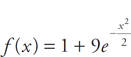
4. B
If we want to find the minimum, we take the derivative and find where the derivative is zero.
f′(x) = 12x2 – 16x
Next, we set the derivative equal to zero and solve for x, in order to find the critical values.
12x2 – 16x = 0
4x(3x – 4) = 0
x = 0 or x = 
![]()
Next, we can use the second derivative test to determine which critical value is a minimum and which is a maximum.
Remember the second derivative test: If the sign of the second derivative at a critical value is positive, then the curve has a local minimum there. If the sign of the second derivative is negative, then the curve has a local maximum there.
We take the second derivative: f′(x) = 24x – 16.
This is negative at x = 0 and positive at x = ![]() . This means that the curve has a relative minimum at x =
. This means that the curve has a relative minimum at x = ![]() , but this value is outside of the interval [−1, 1]. So, in order to find where it has an absolute minimum, we plug the endpoints of the interval into the original equation, and the smaller value will be the answer.
, but this value is outside of the interval [−1, 1]. So, in order to find where it has an absolute minimum, we plug the endpoints of the interval into the original equation, and the smaller value will be the answer.
At x = −1, the value is f(−1) = −11. At x = 1, the value is f (1) = −3.
5. A
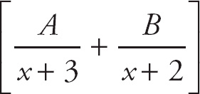
Whenever we have an integrand that is a rational expression, we can often use the method of partial fractions to rewrite the integral in a form in which it’s easy to evaluate.
First, separate the denominator into its two components and place the constants A and B in the numerators of the fractions and the components into the denominators. Set their sum equal to the original rational expression.

Now, we want to solve for the constants A and B. First, multiply through by (x + 3)(x + 2) to clear the denominators.
 = x
= xA(x + 2) + B(x + 3) = x
Now, distribute, then group, the terms on the left side.
Ax + 2A + Bx + 3B = x
Ax + Bx + 2A + 3B = x
(A + B)x + (2A + 3B) = x
In order for this last equation to be true, we need A + B = 1 and 2A + 3B = 0.
If we solve these simultaneous equations, we get A = 3 and B = −2.
Now that we have done the partial fraction decomposition, we can rewrite the original integral as  dx. This is now simple to evaluate.
 = 3 ln |x + 3| − 2 ln |x + 2| + C
Using the rules of logarithms, the answer can be rewritten as  .
.
6. E
Here we need to use the Product Rule, which is: If f(x) = uv, where u and v are both functions of x, then f′(x) =  .
.
We get 
![]() (x2 sin2 x) = 2x sin2 x + x2 (2 sin x cos x).
(x2 sin2 x) = 2x sin2 x + x2 (2 sin x cos x).
This can be simplified to 2x sin2 x + x2 sin 2x.
7. B
The normal line to a curve at a point is perpendicular to the tangent line at the same point. Thus, the slope of the normal line is the negative reciprocal of the slope of the tangent line. We find the slope of the tangent line by finding the derivative and evaluating it at the point.
We need to use the Quotient Rule, which is:
Given y = 
![]() , then:
, then: 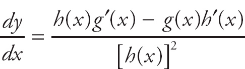 .
.
Here, we have 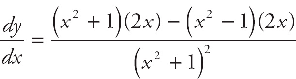 .
.
Next, plug in x = 2 and solve  .
.
Therefore, the slope of the normal line is − 
![]() .
.
8. C
Here we need to use the Product Rule, which is: If f(x) = uv, where u and v are both functions of x, then f′(x) =  .
.
We get h′(x) = f′(x) e g(x) + f(x) [eg(x) g′(x)].
This can be simplified to h′(x) = eg(x) [f′(x) + f(x)g′(x)].
9. D
Here we want to examine the slopes of various pieces of the graph of f(x). Notice that the graph starts with a slope of approximately zero and has a negative slope from x = –∞ to x = −2, where the slope is –∞. Thus, we are looking for a graph of f′(x) that is negative from x = –∞ to x = −2 and undefined at x = −2. Next, notice that the graph of f(x) has a positive slope from x = −2 to x = 2 and that the slope shrinks from ∞ to approximately one and then grows to ∞. Thus, we are looking for a graph of f′(x) that is positive from x = −2 to x = 2 and approximately equal to one at x = 0. Finally, notice that the graph of f(x) has a negative slope from x = 2 to x = ∞, where the slope starts at –∞ and grows to approximately zero. Thus, we are looking for a graph of f′(x) that is negative from x = 2 to x = ∞, where it is approximately zero. Graph (D) satisfies all of these requirements.
10. D
First, expand the integrand:  .
.
Next, evaluate the integral:

11. A
Whenever we have an integral of the form 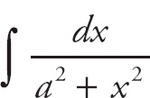 , where a is a constant, the integral is going to be an inverse tangent. So let’s put the integrand into the desired form. Also, we’re going to ignore the limits of integration until after we have done the antidifferentiation.
First, divide the numerator and the denominator by 16: 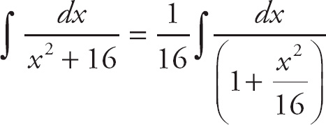 .
.
Next, we do u-substitution. Let u = 
![]() and du =
and du = 
![]() or 4 du = dx.
or 4 du = dx.
Substitute into the integrand: 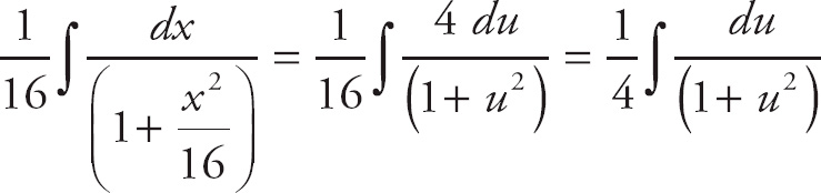 .
.
Evaluate the integral: 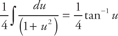 .
.
Substitute back to get  .
.
Now, we can evaluate the function at the limits of integration:

12. B
If we want to find the equation of the tangent line, we first need to find the y-coordinate that corresponds to x = 
![]() . It is y =
. It is y =  .
.
Next, we need to find the derivative of the curve at x = ![]() , using the Chain Rule.
, using the Chain Rule.
We get ![]() = 2 sin x cos x. At x =
= 2 sin x cos x. At x = ![]() ,
, 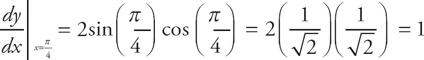 .
.
Now, we have the slope of the tangent line and a point that it goes through. We can use the point-slope formula for the equation of a line, (y – y1) = m(x – x1), and plug in what we have just found. We get 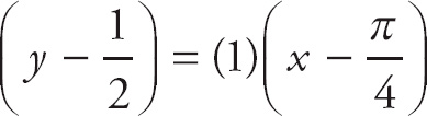 .
.
13. D
A polynomial is continuous everywhere on its domain, so we need to find a value of a such that f(x) is continuous at x = 2. This means that 
![]() f(x) must equal
f(x) must equal 
![]() f(x). In other words, if we plug x = 2 into both pieces of this piecewise function, we need to get the same value.
f(x). In other words, if we plug x = 2 into both pieces of this piecewise function, we need to get the same value.
f(x) =  , so we need 10a + 5 = 8a + 9 and, therefore, a = 2.
14. C
We can evaluate this integral using integration by parts. Here, we let u = x and dv = sin 2x dx. Then du = dx and v = − ![]() cos(2x).
cos(2x).
The rule for integration by parts says that 
![]() u dv = uv −
u dv = uv − ![]() v du.
v du.
Substituting the terms, we get 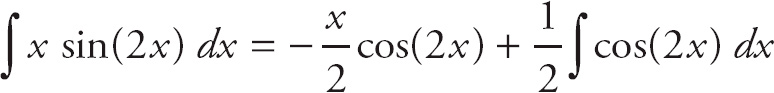
![]() .
.
Now, we integrate the second term, which gives us

15. D
First, try plugging x = −8 into f(x) =  .
.
We get f(x) =  . This does NOT necessarily mean that the limit does not exist. When we get a limit of the form
![]() , we first try to simplify the function by factoring and canceling like terms. Here we get
, we first try to simplify the function by factoring and canceling like terms. Here we get

Now, if we plug in x = −8, we get f(x) =  .
.
16. B
The Taylor series for ex about x = 0 is ex = 1 + x + 
Here, we simply substitute 3 for x in the series, and we get

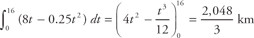
17. E
Because the derivative of velocity with respect to time is acceleration, we have
Now we can plug in the initial condition to solve for the constant.
50 = −10(0) + C
C = 50
Therefore, the velocity function is v(t) = −10t + 50.
Note that the velocity is zero at t = 5.
Next, because the derivative of position with respect to time is velocity, we have
Now, we can plug in the initial condition to solve for the constant.
100 = −5(0)2 + 50(0) + C
C = 100
Therefore, the position function is s(t) = −5t2 + 50t + 100.
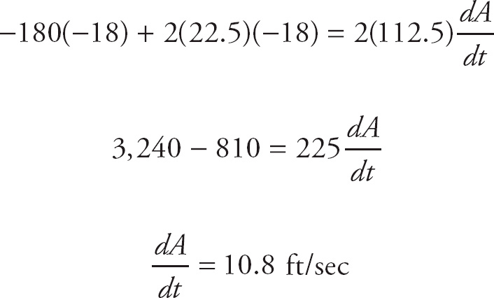
The maximum height occurs when the velocity is zero, so we plug t = 5 into the position function to get s(5) = −5(5)2 + 50(5) + 100 = 225.
18. E
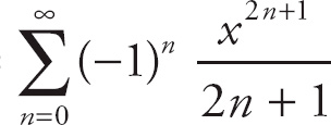
This is the geometric series  . The sum of an infinite series of the form
![]() arn is S =
arn is S = 
![]() . Here, the sum is S =
. Here, the sum is S =  .
.
19. A
Use the Ratio Test to determine the interval of convergence.
We get  =
=  .
.
This converges if  < 1 or −1 <
![]() < 1 and diverges if
< 1 and diverges if  > 1.
> 1.
Thus, the series converges when −2 < x < 8.
Now we need to test whether the series converges at the endpoints of this interval.
When x = 8, we get the series  , which converges, and when x = −2, we get the alternating series
  , which also converges. Thus, the series converges when −2 ≤ x ≤ 8.
20. B
First, let’s graph the curve.

Let’s find the area of the loop in the first quadrant, which is the interval from θ = 0 to θ = 
![]() . We find the area of a polar graph by evaluating A =
. We find the area of a polar graph by evaluating A = 
![]() r2 dθ.
r2 dθ.
Thus, we need to evaluate: A = ![]() sin2 (2θ) dθ.
sin2 (2θ) dθ.
Next, we need to do a trigonometric substitution to evaluate this integral. Recall that cos 2θ = 1 – 2 sin2 θ. We can rearrange this to obtain sin2 θ =  , or in this case, sin2 2θ =
  .
.
Thus, we can rewrite the integral: A = 
![]() .
.
Now we can evaluate this integral.

Now we evaluate the integral at the limits of integration.

21. C
In order to find the average value, we use the Mean Value Theorem for integrals, which says that the average value of f(x) on the interval [a, b] is 
![]() f(x) dx.
f(x) dx.
Here we have  sec2 x dx.
Next, recall that: ![]() = tan x = sec2 x.
= tan x = sec2 x.
We evaluate the integral:  =
=  .
.
Next, we need to do a little algebra. Get a common denominator for each of the two expressions.

We can simplify this to  .
.
22. A
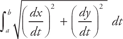
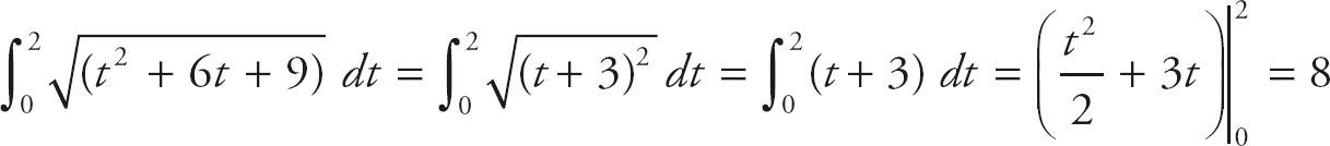
We can find the length of a parametric curve on the interval [a, b] by evaluating the integral.
First, we take the derivatives: ![]() = t and =
= t and = 
![]() .
.
Now, square the derivatives:  = t2 and
  = 6t + 9.
Now, we plug this into the formula, and we get
23. D
A function is decreasing on an interval where the derivative is negative.
The derivative is f′(x) = 4x3 + 12x2.
Next, we want to determine on which intervals the derivative of the function is positive and on which it is negative. We do this by finding where the derivative is zero.
4x3 + 12x2 = 0
4x2 (x + 3) = 0
x = −3 or x = 0
We can test where the derivative is positive and negative by picking a point in each of the three regions –∞ < x < −3, −3 < x < 0, and 0 < x < ∞, plugging the point into the derivative, and seeing what the sign of the answer is. You should find that the derivative is negative on the interval –∞ < x < −3.
24. C
Let’s take a look at each series (the series are duplicated below).
I. 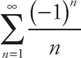 II.
II. 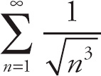 III.
III. 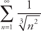
Series I: You might recognize this as the alternating harmonic series, which converges. If you don’t, use the alternating series test, which says, in order for an alternating series 
![]() (− 1)n an to converge: (1) an+1 < an; (2)
(− 1)n an to converge: (1) an+1 < an; (2) 
![]() an = 0; and (3) an > 0. This series satisfies these conditions, so it converges.
an = 0; and (3) an > 0. This series satisfies these conditions, so it converges.
Series II: We can rewrite this series as  , which is a p-series. A p-series is a series of the form
  , which converges if p > 1 and diverges if p < 1. Thus, this series converges.
Series III: We can rewrite this series as  , which is also a p-series. Because p < 1, this series diverges.
25. A
We can solve this differential equation by separation of variables.
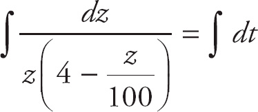
The integral on the right is trivial. We get t + C.
The one on the left will require the Method of Partial Fractions. First, separate the denominator into its two components and place the constants A and B in the numerators of the fractions and the components into the denominators. Set their sum equal to the original rational expression:  .
.
Now, we want to solve for the constants A and B. First, multiply through by  to clear the denominators.

Now, distribute, then group, the terms on the left side.

In order for this last equation to be true, we need 4A = 1 and B − 
![]() = 0.
= 0.
If we solve these simultaneous equations, we get A = 
![]() and B =
and B = 
![]() .
.
Now that we have done the partial fraction decomposition, we can rewrite the original integral as  . This is now simple to evaluate.
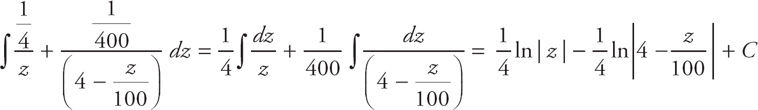
We can rewrite this with the laws of logarithms to get

Thus, the solution to the differential equation is ln = t + C. We will need to do some algebra to rearrange the equation. First, exponentiate both sides to base e.
= et+CThen, because et+C = eteC, and because eC is a constant, we get = Cet.
Next, raise both sides to the fourth power:  = Ce4t.
Invert both sides:  = Ce−4t.
Break the left side into two fractions:  = Ce−4t.
Add 
![]() to both sides:
to both sides:  .
.
Invert both sides (again): 
![]() .
.
Finally: z(t) = 
![]() (Whew!).
(Whew!).
Now, we can take the limit: 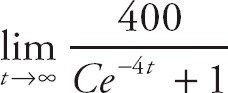
![]() = 400.
= 400.
26. D

The slope field shown above corresponds to which of the following differential equations?
Notice that the slope of the differential equation is zero (horizontal tangent) at the origin. This eliminates answer choices (A) and (B) because they are undefined at the origin (so they would show a vertical tangent there). Next, notice that the slope is positive at (1, 0). This eliminates answer choice (C), which is zero on both axes. Finally, notice that the slope is negative at (0, 1), which eliminates answer choice (E), which is positive there.
27. E
The Mean Value Theorem for derivatives says that, given a function f(x) which is continuous and differentiable on [a, b], then there exists some value c on (a, b) where
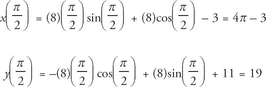
Here, we have  = 19.
= 19.
Plus, f′(c) = 3c2 – 6, so we simply set 3c2 – 6 = 19. If we solve for c, we get c = ± 
![]() . Both of these values satisfy the Mean Value Theorem for derivatives, but only the positive value, c =
. Both of these values satisfy the Mean Value Theorem for derivatives, but only the positive value, c = ![]() , is in the interval.
, is in the interval.
28. E
If we want to find where g(x) is a minimum, we can look at g′(x). The Second Fundamental Theorem of Calculus tells us how to find the derivative of an integral: 
![]() f(t) dt = f(x), where c is a constant. Thus, g′(x) = f(x). The graph of f is zero at x = 0, x = 2, and x = 4. We can eliminate x = 0 because we are looking for a positive value of x. Next, notice that f is negative to the left of x = 4 and positive to the right of x = 4. Thus, g(x) has a minimum at x = 4.
f(t) dt = f(x), where c is a constant. Thus, g′(x) = f(x). The graph of f is zero at x = 0, x = 2, and x = 4. We can eliminate x = 0 because we are looking for a positive value of x. Next, notice that f is negative to the left of x = 4 and positive to the right of x = 4. Thus, g(x) has a minimum at x = 4.
We also could have found the answer geometrically. The function g(x) = 
![]() f(t) dt is called an accumulation function and stands for the area between the curve and the x-axis to the point x. Thus, the value of g grows from x = 0 to x = 2. Then, because we subtract the area under the x-axis from the area above it, the value of g shrinks from x = 2 to x = 4. The value begins to grow again after x = 4.
f(t) dt is called an accumulation function and stands for the area between the curve and the x-axis to the point x. Thus, the value of g grows from x = 0 to x = 2. Then, because we subtract the area under the x-axis from the area above it, the value of g shrinks from x = 2 to x = 4. The value begins to grow again after x = 4.
29. A
The slope of the tangent line is the derivative of the function. We get f′(x) = 3e3x. Now we set the derivative equal to 2 and solve for x.
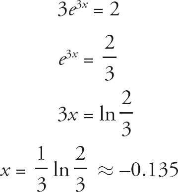
(Remember to round all answers to three decimal places on the AP exam.)
30. D
We need to use logarithmic differentiation to find the derivative. First, take the log of both sides: ln y = ln[(sinx)ex].
Next, on the right side, put the power in front of the log: ln y = ex ln(sin x)
Next, take the derivative of both sides:  .
.
This can be simplified to 
![]() = ex ln(sin x) + ex cot x.
= ex ln(sin x) + ex cot x.
Multiply both sides by y: ![]() = y[ex ln(sin x) + ex cot x].
= y[ex ln(sin x) + ex cot x].
Substitute y = (sin x)ex for y on the right side: ![]() = (sin x)ex [ex ln(sin x) + ex cot x].
= (sin x)ex [ex ln(sin x) + ex cot x].
Finally, factor out ex to obtain ![]() = ex (sin)ex [ln(sin x) + cot x].
= ex (sin)ex [ln(sin x) + cot x].
31. B
The formula for the perimeter of a square is P = 4s, where s is the length of a side of the square.
If we differentiate this with respect to t, we get  . We plug in
![]() = 0.4, and we get
= 0.4, and we get 
![]() = 4(0.4) = 1.6.
= 4(0.4) = 1.6.
The formula for the area of a square is A = s2. If we solve the perimeter equation for s in terms of P and substitute it into the area equation, we get

If we differentiate this with respect to t, we get 
![]() .
.
Now we plug in ![]() = 1.6 and we get
= 1.6 and we get 
![]() = 0.2P.
= 0.2P.
32. A
The acceleration vector is the second derivative of the position vector (the velocity vector is the first derivative).
The velocity vector of this particle is (2 cos 2t, 2 sin t cos t).
This can be simplified to (2 cos 2t, sin 2t).
The acceleration vector is: (−4 sin 2t, 2 cos 2t)
33. B
The velocity of the mass is the first derivative of the height: v(t) = 8 sin(2t).
Now graph the equation to find how many times the graph of v(t) crosses the t-axis between t = 0 and t = 2. Or you should know that this is a sine graph with an amplitude of 8 and a period of π, which will cross the t-axis once on the interval at t = ![]() .
.
34. D
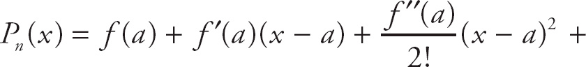
Notice how this limit takes the form of the definition of the derivative, which is
Here, if we think of f(x) as tan−1 x, then this expression gives the derivative of tan−1 x at the point x = 1.
The derivative of tan−1 x is f′(x) = 
![]() . At x = 1, we get
. At x = 1, we get
f′(1) = ![]()
35. C
The Trapezoid Rule enables us to approximate the area under a curve with a fair degree of accuracy. The rule says that the area between the x-axis and the curve y = f(x), on the interval [a, b], with n trapezoids, is
 [y0 + 2y1 + 2y2 + 2y3 + … + 2yn−1 + yn]
Using the rule here, with n = 4, a = 0, and b = 3, we get

36. D
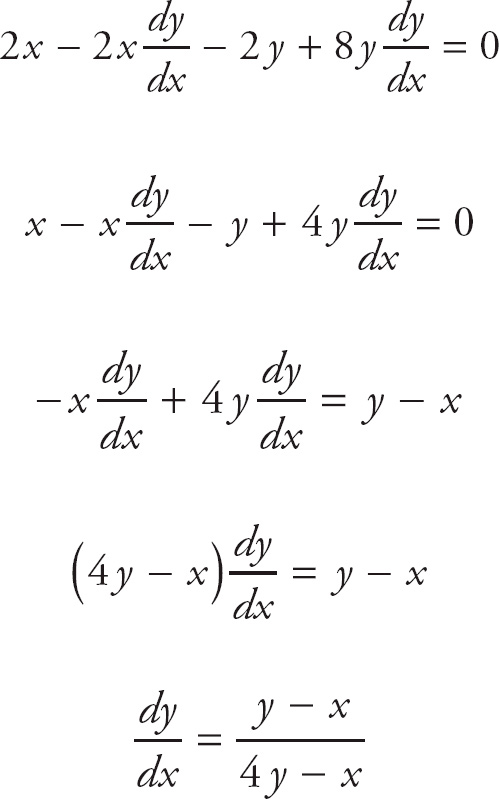
Use implicit differentiation to find ![]() : x2
: x2 ![]() + 2xy + 2x = 2y
+ 2xy + 2x = 2y ![]() .
.
Now we want to isolate ![]() , which will take some algebra.
, which will take some algebra.
First, put all of the terms containing ![]() on one side of the equals sign and all of the other terms on the other side: 2xy + 2x = 2y
on one side of the equals sign and all of the other terms on the other side: 2xy + 2x = 2y ![]() − x2
− x2 ![]() .
.
Next, factor ![]() out of the right hand side: 2xy + 2x =
out of the right hand side: 2xy + 2x = ![]() (2y – x2).
(2y – x2).
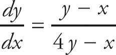
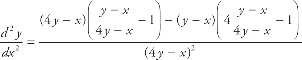
Finally, divide both sides by (2y – x2) to isolate ![]() :
: 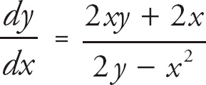 .
.
At (1, 1), we get  = 4.
= 4.
Now, we can find the second derivative by again performing implicit differentiation.

At (1, 1), we get 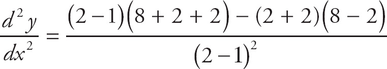 =
= 
![]() .
.
37. D
Because the integral of a function can be interpreted as the area between the function and the curve, we can say that 
![]() , where c is a point in the interval (a, b). Here we have
, where c is a point in the interval (a, b). Here we have 
![]() . We can rearrange this to:
. We can rearrange this to: 
![]() . This means that a − b =
. This means that a − b = 
![]() f(x) dx. Finally, we know that
f(x) dx. Finally, we know that 
![]() .
.
38. A
The Second Fundamental Theorem of Calculus tells us how to find the derivative of an integral: 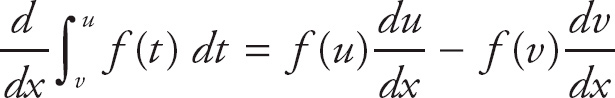
![]() , where u and v are functions of x.
, where u and v are functions of x.
Here we can use the theorem to get 
![]() cos t dt = 5 cos 5x − 2 cos2 x.
cos t dt = 5 cos 5x − 2 cos2 x.
39. B
We are given that sin x = x –  + …
+ …
Here, we simply substitute 0.4 for x in the series, and we get
 + …
+ …Find the value on your calculator. Keep adding terms until you get four decimal places of accuracy. You should get: sin(0.4) = 0.3894. If you got only 0.3893, you didn’t use enough terms (you need to use the fifth power term).
40. E
First, we graph the curves.

We can find the volume by taking a vertical slice of the region. The formula for the volume of a solid of revolution around the y-axis, using a vertical slice bounded from above by the curve f(x) and from below by g(x), on the interval [a, b], is

The upper curve is y = e–x, and the lower curve is y = sin x.
Next, we need to find the point(s) of intersection of the two curves with a calculator (Good luck doing it by hand!), which we do by setting them equal to each other and solving for x. You should get approximately: x = 0.589 (remember to round to three decimal places on the AP exam).
Thus, the limits of integration are x = 0 and x = 0.589.
Now, we evaluate the integral.
We can evaluate this integral by hand but, because we will need a calculator to find the answer, we might as well use it to evaluate the integral.
We get ![]() (e−2x − sin2 x) dx = 0.888 (rounded to three decimal places).
(e−2x − sin2 x) dx = 0.888 (rounded to three decimal places).
41. C
We can use Euler’s Method to find an approximate answer to the differential equation. The method is quite simple. First, we need a starting point, (x0, y0) and an initial slope, y′0. Next, we use increments of h to come up with approximations. Each new approximation will use the following rules:
xn = xn – 1 + h
yn = yn – 1 + h • y′n − 1
Repeat for n = 1, 2, 3, …
We are given that the curve goes through the point (2, 6). We will call the coordinates of this point x0 = 2 and y0 = 6. The slope is found by plugging these coordinates into y′ = 2y – 4x, so we have an initial slope of y′0 = 4.
Now, we need to find the next set of points.
Step 1: Increase x0 by h to get x1: x1 = 2.2.
Step 2: Multiply h by y′0 and add to y0 to get y1: y1 = 6 + 0.2(4) = 6.8.
Step 3: Find y′1 by plugging x1 and y1 into the equation for y′.
y′1 = 2(6.8) – 4(2.2) = 4.8
Repeat until we get to the desired point (in this case x = 3).
Step 1: Increase x1 by h to get x2: x2 = 2.4.
Step 2: Multiply h by y′1 and add to y1 to get y2: y2 = 6.8 + 0.2(4.8) = 7.76.
Step 3: Find y′2 by plugging x2 and y2 into the equation for y′.
y′2 = 2(7.76) – 4(2.4) = 5.92
Step 2: y3 = y2 + h(y′2): y3 = 7.76 + 0.2(5.92) = 8.944
Step 3: y′3 = 2(y3) – 4(x3): y′3 = 2(8.944) – 4(2.6) = 7.488
Step 1: x4 = x3 + h: x4 = 2.8
Step 2: y4 = y3 + h(y′3): y4 = 8.944 + 0.2(7.488) = 10.4416
Step 3: y′4 = 2(y4) – 4(x4): y′4 = 2(10.4416) – 4(2.8) = 9.6832
Step 1: x5 = x4 + h: x5 = 3
Step 2: y5 = y4 + h(y′4): y5 = 10.4416 + 0.2(9.6832) = 12.378
42. B
First, break up the integrand: ![]() sec4 x dx =
sec4 x dx = ![]() (sec2 x)(sec2 x) dx.
(sec2 x)(sec2 x) dx.
Next, use the trig identity 1 + tan2 x = sec2 x to rewrite the integral.

We can evaluate these integrals separately.
The left one is easy: ![]() sec2 x dx = tan x + C.
sec2 x dx = tan x + C.
We will use u-substitution for the right one. Let u = tan x and du = sec2 x dx. Then, substitute into the integral and integrate: 
![]() .
.
Now, substitute back: 
![]() tan3 x + C.
tan3 x + C.
Combine the two integrals to get tan x + ![]() tan3 x + C.
tan3 x + C.
43. E
We find ![]() cot x dx by rewriting the integral as
cot x dx by rewriting the integral as 
![]() dx. Then we use u-substitution. Let u = sin x and du = cos x. Substituting, we can get
dx. Then we use u-substitution. Let u = sin x and du = cos x. Substituting, we can get
Then, substituting back, we get ln(sin x) + C. (We can get rid of the absolute value bars because sine is always positive on the interval.) Next, we use  = 1 to solve for C.
We get

Thus, f(x) = ln(sin x) + 1.693147.
At x = 1, we get f (1) = ln(sin1) + 1.693147 = 1.521 (rounded to three decimal places).
44. C
We solve an integral of the form 
![]() by performing the trig substitution x = asin θ. Here we will use x = 2sin θ, which means that dx = 2 cos θ dθ. We get:
by performing the trig substitution x = asin θ. Here we will use x = 2sin θ, which means that dx = 2 cos θ dθ. We get: 
![]() . Next, factor out the 4:
. Next, factor out the 4: 
![]() cos θ dθ.
cos θ dθ.
Next, simplify the radicand: 
![]() cos θ dθ., which gives us 4
cos θ dθ., which gives us 4 ![]() cos2 θ dθ. Now, we need to use another trig identity. Recall that cos 2θ = 2cos2 θ – 1, which can be rewritten as cos2 θ =
cos2 θ dθ. Now, we need to use another trig identity. Recall that cos 2θ = 2cos2 θ – 1, which can be rewritten as cos2 θ =  .
.
Now, we can rewrite the integral:  .
.
Integrate: 2 ![]() (1 + cos 2θ) dθ = 2θ + sin 2θ + C.
(1 + cos 2θ) dθ = 2θ + sin 2θ + C.
Now, we have to substitute back.
Because x = 2 sin θ, we know that θ = sin−1 
![]() and that cos θ =
and that cos θ =  .
.
This gives us 2θ + sin 2θ + C = 2 sin−1![]() +
+ 
![]() + C.
+ C.
45. E
Hooke’s law says that the force needed to compress or stretch a spring from its natural state is F = kx, where k is the spring constant. We can find the value of k from the initial information, namely F = 250 N for a stretch of 5 m. Thus, we can solve to find the value of k: k = 250/5 = 50 N/m.
We find the work done by a variable force along the x-axis from x = a to x = b by evaluating the integral for the Work, W = 
![]() F(x) dx.
F(x) dx.
Using the information we have, W = 
![]() = 1,225 N.
= 1,225 N.