
Go provides two sizes of floating-point numbers, float32 and
float64.
Their arithmetic properties are governed by the IEEE 754 standard
implemented by all modern CPUs.
Values of these numeric types range from tiny to huge.
The limits of floating-point values can be found in the math
package.
The constant math.MaxFloat32, the largest float32, is
about 3.4e38, and math.MaxFloat64 is about 1.8e308.
The smallest
positive values are near 1.4e-45 and 4.9e-324, respectively.
A float32 provides approximately six decimal digits of precision, whereas
a float64 provides about 15 digits; float64 should be preferred for
most purposes because float32 computations accumulate error
rapidly unless one is quite careful, and the smallest positive integer that
cannot be exactly represented as a float32 is not large:
var f float32 = 16777216 // 1 << 24
fmt.Println(f == f+1)    // "true"!
Floating-point numbers can be written literally using decimals, like this:
const e = 2.71828 // (approximately)
Digits may be omitted before the decimal point (.707) or after it
(1.). Very small or very large numbers are better
written in scientific notation, with the letter e or E preceding
the decimal exponent:
const Avogadro = 6.02214129e23
const Planck   = 6.62606957e-34
Floating-point values are conveniently printed with Printf’s %g verb,
which chooses the most compact representation that has adequate precision,
but for tables of
data, the %e (exponent) or %f (no exponent) forms may be more
appropriate.
All three verbs allow field width and numeric precision to be
controlled.
for x := 0; x < 8; x++ {
    fmt.Printf("x = %d ex = %8.3f\n", x, math.Exp(float64(x)))
}
The code above prints the powers of e with three decimal digits of precision, aligned in an eight-character field:
x = 0   ex =    1.000
x = 1   ex =    2.718
x = 2   ex =    7.389
x = 3   ex =   20.086
x = 4   ex =   54.598
x = 5   ex =  148.413
x = 6   ex =  403.429
x = 7   ex = 1096.633
In addition to a large collection of the usual mathematical functions,
the math package has functions for creating and detecting the
special values defined by IEEE 754: the positive and negative
infinities, which represent numbers of excessive magnitude and the
result of division by zero; and NaN (“not a number”), the result of
such mathematically dubious operations as 0/0 or Sqrt(-1).
var z float64
fmt.Println(z, -z, 1/z, -1/z, z/z) //  "0 -0 +Inf -Inf NaN"
The function math.IsNaN tests whether its argument is a not-a-number
value, and math.NaN returns such a value. It’s
tempting to use NaN as a sentinel value in a numeric computation, but
testing whether a specific computational result is equal to NaN is
fraught with peril because any comparison with NaN always yields false:
nan := math.NaN()
fmt.Println(nan == nan, nan < nan, nan > nan) // "false false false"
If a function that returns a floating-point result might fail, it’s better to report the failure separately, like this:
func compute() (value float64, ok bool) {
    // ...
    if failed {
        return 0, false
    }
    return result, true
}
The next program illustrates floating-point graphics
computation. It plots a function of two variables z = f(x, y)
as a wire mesh 3-D surface, using Scalable Vector Graphics (SVG),
a standard XML notation for line drawings.
Figure 3.1 shows an example of its output
for the function sin(r)/r, where r is
sqrt(x*x+y*y).
// Surface computes an SVG rendering of a 3-D surface function.
package main

import (
    "fmt"
    "math"
)

const (
    width, height = 600, 320            // canvas size in pixels
    cells         = 100                 // number of grid cells
    xyrange       = 30.0                // axis ranges (-xyrange..+xyrange)
    xyscale       = width / 2 / xyrange // pixels per x or y unit
    zscale        = height * 0.4        // pixels per z unit
    angle         = math.Pi / 6         // angle of x, y axes (=30°)
)

var sin30, cos30 = math.Sin(angle), math.Cos(angle) // sin(30°), cos(30°)

func main() {
    fmt.Printf("<svg xmlns='http://www.w3.org/2000/svg' "+
        "style='stroke: grey; fill: white; stroke-width: 0.7' "+
        "width='%d' height='%d'>", width, height)
    for i := 0; i < cells; i++ {
        for j := 0; j < cells; j++ {
            ax, ay := corner(i+1, j)
            bx, by := corner(i, j)
            cx, cy := corner(i, j+1)
            dx, dy := corner(i+1, j+1)
            fmt.Printf("<polygon points='%g,%g %g,%g %g,%g %g,%g'/>\n",
                ax, ay, bx, by, cx, cy, dx, dy)
        }
    }
    fmt.Println("</svg>")
}

func corner(i, j int) (float64, float64) {
    // Find point (x,y) at corner of cell (i,j).
    x := xyrange * (float64(i)/cells - 0.5)
    y := xyrange * (float64(j)/cells - 0.5)

    // Compute surface height z.
    z := f(x, y)

    // Project (x,y,z) isometrically onto 2-D SVG canvas (sx,sy).
    sx := width/2 + (x-y)*cos30*xyscale
    sy := height/2 + (x+y)*sin30*xyscale - z*zscale
    return sx, sy
}

func f(x, y float64) float64 {
    r := math.Hypot(x, y) // distance from (0,0)
    return math.Sin(r) / r
}
Notice that the function corner returns two values, the coordinates
of the corner of the cell.
The explanation of how the program works requires only basic geometry, but it’s fine to skip over it, since the point is to illustrate floating-point computation. The essence of the program is mapping between three different coordinate systems, shown in Figure 3.2. The first is a 2-D grid of 100×100 cells identified by integer coordinates (i, j), starting at (0, 0) in the far back corner. We plot from the back to the front so that background polygons may be obscured by foreground ones.
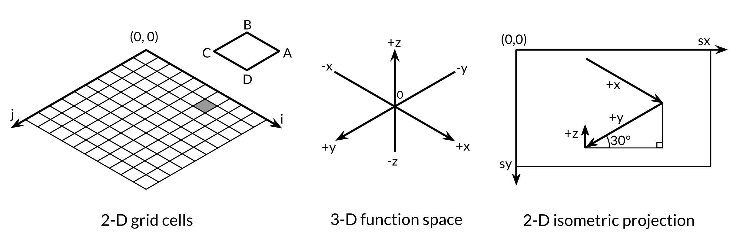
Figure 3.2. Three different coordinate systems.
The second coordinate system is a mesh of 3-D floating-point coordinates (x,
y, z), where x and y are linear functions
of i and j, translated so that the origin is in the center,
and scaled by the constant xyrange. The height z is the value of the
surface function f (x, y).
The third coordinate system is the 2-D image canvas, with (0, 0) in the top left corner. Points in this plane are denoted (sx, sy). We use an isometric projection to map each 3-D point (x, y, z) onto the 2-D canvas. A point appears farther to the right on the canvas the greater its x value or the smaller its y value. And a point appears farther down the canvas the greater its x value or y value, and the smaller its z value. The vertical and horizontal scale factors for x and y are derived from the sine and cosine of a 30° angle. The scale factor for z, 0.4, is an arbitrary parameter.
For each cell in the 2-D grid, the main function computes the coordinates on the image canvas of the four corners of the polygon ABCD, where B corresponds to (i, j) and A, C, and D are its neighbors, then prints an SVG instruction to draw it.
Exercise 3.1:
If the function f returns a non-finite float64 value,
the SVG file will contain invalid <polygon>
elements (although many SVG renderers handle this gracefully).
Modify the program to skip invalid polygons.
Exercise 3.2:
Experiment with visualizations of other functions from the math package.
Can you produce an egg box, moguls, or a saddle?
Exercise 3.3:
Color each polygon based on its height, so that the peaks are colored
red (#ff0000) and the valleys blue (#0000ff).
Exercise 3.4:
Following the approach of the Lissajous example in Section 1.7,
construct a web server that computes surfaces and writes SVG data to
the client.
The server must set the Content-Type header like this:
w.Header().Set("Content-Type", "image/svg+xml")
(This step was not required in the Lissajous example because the server uses standard heuristics to recognize common formats like PNG from the first 512 bytes of the response, and generates the proper header.) Allow the client to specify values like height, width, and color as HTTP request parameters.