Chapter 2: The Arithmetic Foundations of a Neural Network
Before we can explore advanced concepts and practical examples of Deep learning, we must first familiarize ourselves with the mathematical ideas that are the foundations of the Neural networks making up the Deep learning system. These mathematical concepts include:
- Tensors
- Tensor operations
- Differentiation
- Gradient descent, and many more.
The main focus of this chapter will be to structure our discussion to encompass the core ideas and workings of these mathematical concepts, all while keeping our discussion from becoming too technical. In other words, this chapter will cater to the needs of the readers by building up an intuitive understanding of these important concepts and refrain from using mathematical notations. This way, the readers who do not have over the top mathematical prowess can also benefit and build a good understanding relating to the topic.
This chapter is essential to understand as it is the blueprint for understanding the practical examples, which will be detailed in the later sections of this book. As such, the chapter will take off by introducing a practical example of a Neural network, and then we will work our way through it to understand the corresponding concepts.
A Peek into a Neural Network
For our example, we will discuss a Neural network that utilizes the “Keras” library (a Python library to be exact). The main concern of this Neural network is learning on how to classify handwritten digits. For now, it is not necessary to be familiar with the Keras library as we will discuss the details of every element of this example in the following chapters. Right now, it is necessary to understand the fundamentals of what makes up this Neural network.
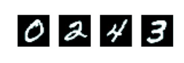
In this example of a Neural network, we are concerned with classifying handwritten digits. These handwritten digits are in the form of grayscale images with a resolution of 28x28 pixels. The job of the Neural network is to classify these images of handwritten digits into their respective categories of 0 to 9 (in short, classify them into 10 categories). The dataset which will be used in this example is none other than the classic MNIST dataset because this specific dataset has been intensively studied in the Machine-learning community, making it a suitable choice for our example. Hence, solving this classic dataset can also be considered as making your very first program (Hello World!). Below are sample digits that are taken from the MNIST dataset.
One more reason why we have used the Keras Python library in our demonstrative Neural network is that the MNIST dataset (set of four NumPy Arrays) comes preloaded with this library.
The following lines of code shown below depict how you can load the MNIST dataset into the Keras library:
from keras.datasets import mnist
(train_images, train_labels), (test _images, test_labels) = mnist.load_data()
The train_images and train_labels are basically the resources which the model will use as learning material, and later onwards, it will be tested on the test_images and test_labels. In other words, the MNIST dataset includes a training set and a test set.
The learning process works in this way that the model establishes a mirrored correspondence to the images (encoded as NumPy arrays) and the labels (array of digits).
The resulting training data obtained would look like this:
>>> train_images.shape
(60000, 28, 28)
>>> len(train_labels)
60000
>>> train_labels
array([5, 0, 4, ..., 5, 6, 8], dtype=uint8)
Similarly, the corresponding test data is:
>>> test_images.shape
(10000, 28, 28)
>>> len(test_labels)
10000
>>> test_labels
array([7, 2, 1, ..., 4, 5, 6], dtype=uint8)
Now proceeding to explain the workflow of the model as it trains itself using the training set and later tests itself through the test set. As it is obvious, we are providing the Neural network with data to train it by using the train_images and train_labels from the training set of the MNIST dataset. After the Neural network has learned how to identify and associate the corresponding images and labels, we move on to testing its capability by exposing it to the data from test_images and ask it to predict what labels do these images correspond to. After this, the predictions produced by the Neural network are matched with the test_labels to check whether they are accurate or completely off the mark.
Now, we will proceed to build the Neural network even further. The architecture of the network will look like this:
from keras import models
from keras import layers
network = models.Sequential()
network.add(layers.Dense(512, activation='relu', input_shape=(28 * 28,)))
network.add(layers.Dense(10, activation='softmax'))
From the above Neural network architecture, we get to see the following important terms:
-
Layers
: The layer is considered as the most important building block of any Neural network. Layers are basically modules that are concerned with data processing, and they act as filters for data, in the sense that when a layer processes data, the resulting data is in a form that is more useful and effective than it previously was. In other words, the specific function of a layer is to take the sample data and extract the representations from it. In short, layers are essentially just data filters.
-
Data Distillation
: Data distillation is a progressive process that takes shape when multiple simple layers are chained together.
-
Dense Layers
: Dense layers are basically neural layers that are completely connected (densely connected).
-
Softmax Layer
: The network sequence shown above details a 10-way softmax layer, which is actually a probability layer, i.e., it functions to return an array that consists of 10 probability scores. Each of these 1o scores gives us a probability of how the active (current) digit is actually part of one of the 10 digit classes.
Even now, our network is still not ready for training. We still need three vital elements that will essentially make up the compilation step:
-
Loss Function
: This details the way through which the network will be able to gain an idea of its performance, and in this way, it will be able to shift the direction of its work towards the right direction.
-
Optimizer
: This is a mechanism that allows the network to update itself corresponding to two elements: the analyzed data and the loss function.
-
Metrics
: These metrics are to be used for monitoring the network during its training and testing stages, and the main concern of this step is the accuracy of the Neural network by which it can correctly classify the images.
Although the purpose of the loss function and optimizer may seem unclear right now, however, the practical examples and explanations in the coming chapters will address their workings in more detail.
Now, we will implement the compilation step into our Neural network:
network.compile(optimizer='rmsprop',
loss='categorical_crossentropy',
metrics=['accuracy'])
However, our Neural network is still not ready for training. There are still quite a few steps required before we can proceed to train the method in Keras by using a method known as “fit” (which will be explained shortly). Hence, the first thing we need to do here is to pre-process the data. This is done by reshaping the data into a form that is expected by the network. In addition, we also need to scale the data to bring all the corresponding values into an interval of [0, 1]. For example, consider the very first example we discussed in this chapter, if you look at it closely, you will notice that the training images are a unit8 type and not only that, but they are also stored in an array of (6000, 28, 28). Moreover, the values were unscaled and in an interval of [0, 255]. Hence, we will transform this example in the following parameters:
- Array type from unit8 to float32
- Array shape from (6000, 28, 28) to (6000, 28 * 28)
- Values in [0, 255] interval to [0, 1] interval
The lines of code to do this are:
train_images = train_images.reshape((60000, 28 * 28))
train_images = train_images.astype('float32') / 255
test_images = test_images.reshape((10000, 28 * 28))
test_images = test_images.astype('float32') / 255
The last step left to do is that the labels are needed to be encoded categorically, which can be done as shown below:
from keras.utils import to_categorical
train_labels = to_categorical(train_labels)
test_labels = to_categorical(test_labels)
Finally, we are now all set up to proceed with training the Neural network by using the Keras library. To do this, we will call to a method known as the “network.fit”. This basically fits the network’s model to the corresponding training data, as shown below:
>>> network.fit(train_images, train_labels, epochs=5, batch_size=128)
Epoch 1/5
60000/60000 [==============================] - 9s - loss: 0.2524 - acc: 0.9273
Epoch 2/5
51328/60000 [========================>.....] - ETA: 1s - loss: 0.1035 - acc: 0.9692
Now, if we take a closer look at the result, we can see that two quantities are being displayed in the training session. These quantities of the network over the training data respectively are:
In the training session, we observe an accuracy of 98.9%. We will now proceed to determine whether the model performs similarly on the test dataset.
>>> test_loss, test_acc = network.evaluate(test_images, test_labels)
>>> print('test_acc:', test_acc)
test_acc: 0.9785
The accuracy shown in the test session is actually lower than the accuracy shown in the training session, i.e., 97.8% and 98.9%, respectively. This gap of accuracy is termed as “overfitting.” This reinforces the fact that the Machine-learning models do not perform at the same level when exposed to new data as compared to their performance with the training dataset.
Data Attributes of Neural Networks
In this section, we will be focusing on the attributes of the most common data structure, tensors
. Tensors are basically data storage containers as the very NumPy arrays in which multi-dimensional data is stored itself called a tensor. The type of data stored in tensors is usually numerical data. Hence it is also technically plausible to consider tensors as storage containers for numbers. Also, it is important to remember that in the context of a tensor, a dimension is basically referring to an axis.
Based on the dimensions, there are four common types of tensors used in Machine learning, namely:
- Scalars (0D tensors)
- Vectors (1D tensors)
- Matrices (2D tensors)
- 3D tensors and higher dimensional tensors
Scalars (0D tensors)
Scalars are basically those tensors that only have one number stored. Other names for scalars are scalar tensors, 0-dimensional tensor, or 0D tensor. Scalar tensors are represented by both floath32 and float64 numbers in NumPy. Moreover, a “rank” basically refers to the number of axes that are within a tensor. We can also find out the number of axes within a NumPy tensor by using an attribute known as the ndim
attribute. (Remember that as Scalars are zero-dimensional, their ndim attribute will always be 0). Below is an example of a NumPy scalar:
>>> import numpy as np
>>> x = np.array(12)
>>> x
array(12)
>>> x.ndim
0
Vectors (1D tensors)
Vectors are those tensors that contain an array of numbers while having only one axis, hence the name “1D tensor”. A NumPy vector is shown below:
>>> x = np.array([18, 5, 9, 11])
>>> x
array([18, 5, 9, 11])
>>> x.ndim
1
Upon careful inspection, we can see that a vector consists of 5 entries and because of this we can call such a vector a 5-dimensional vector. It is important to note that a 5-dimensional vector is not the same as a 5D tensor, as a dimension can both refer to the number of entries and the number of axes in a tensor. As such, it is when faced with such confusing scenarios, it is better to refer to a 5D tensor as a tensor of rank 5).
Matrices (2D tensors)
Matrices are those tensors that contain an array of vectors. A matrix is also known as a 2D tensor because it consists of two axes (the rows and columns). A NumPy matrix is shown below:
>>> x = np.array([[2, 52, 8, 22, 9],
[4, 2 12, 23, 5],
[8, 11, 33, 98, 5]])
>>> x.ndim
2
In this example, the horizontal entries (the x-axis) are considered as the rows, for instance, in the above example, the entry [2, 52, 8, 22, 9] is the first axis (the row) and the vertical entry [2, 4, 8] is the second axis (the column).
3D Tensors and Higher-Dimensional Tensors
3D tensors are basically a bunch of matrices packed in such a way that they are visually interpreted as a cube of numbers. For example, a typical 3D tensor looks like this:
>>> x = np.array([[[5, 78, 2, 34, 0],
[6, 79, 3, 35, 1],
[7, 80, 4, 36, 2]],
[[5, 78, 2, 34, 0],
[6, 79, 3, 35, 1],
[7, 80, 4, 36, 2]],
[[5, 78, 2, 34, 0],
[6, 79, 3, 35, 1],
[7, 80, 4, 36, 2]]])
>>> x.ndim
3
Just as how we created a 3D tensors by packing multiple matrices in an array, similarly, we can obtain a 4D tensor by packing multiple 3D tensors in an array and the same process holds for obtaining 5D tensors and so on. Generally we are only required to manipulate tensors from 0D to 4D when using them in deep learning, however, we may also need to go to 5D tensors if we are dealing with the processing of video data.
The Key Attributes of Tensors
Generally, a tensor has three defining key attributes. These attributes are:
-
The Rank
: Rank refers to the number of axes a tensor has. For example, we discussed a Matrix that has two axes; hence it has a rank of 2. Similarly, a 3D tensor has three axes, so it has a rank of 1. Ranks are referred to as ndim
in the NumPy library.
-
Shape
: A shape is the computing structure that defines the number of dimensions that a tensor has along each axis. For instance, consider the above examples of different types of tensors. A scalar tensor has no dimension; hence its shape is (), a vector has only one dimension, so its shape is (3, ) and a matrix has two dimensions, so its shape is (2, 6). A 3D tensor has three dimensions; hence, it has a shape of (1, 2, 3) and so on.
-
Data Type
: Data type is commonly referred to as “dtype,” specifically in the Python libraries. As the name suggests, this refers to the very type of data that is being stored in the tensor itself, for example, unit8, float32, and float64 are all data types.
Let’s take this discussion a bit further and explain these attributes more clearly by looking at a demonstration of the data we processed previously in our MNIST example. To start, we will first load up the MNIST data set by:
from keras.datasets import mnist
(train_images, train_labels), (test_images, test_labels) = mnist.load_data()
Now, by using the ndim
attribute, we will proceed to display the number of axes that the tensor (train_images) currently has:
>>> print(train_images.ndim)
3
Now to display the shape attribute of the tensor:
>>> print(train_images.shape)
(30000, 18, 18)
And finally, the dtype
attribute or the data type of the tensor:
>>> print(train_images.dtype)
uint8
From the above results, we come to know that the tensor is, in fact, a 3D tensor, specifically of 8-bit integers. Furthermore, the shape of this tensor is that of an array of 30000 matrices with 18x8 integers.
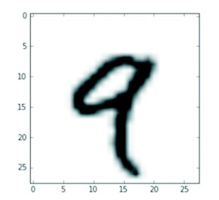
We can also display any digit within this 3D tensor. This can be done by utilizing the Matplotlib library. For instance, the example below depicts the lines through which we are displaying the fourth digit in our 3D tensor:
digit = train_images[4]
import matplotlib.pyplot as plt
plt.imshow(digit, cmap=plt.cm.binary)
plt.show()
Gearing the Neural Network through Tensor Operations
Technically, if we begin to break down any computer program to its fundamentals, then we will ultimately come down to a mere set of binary operations on binary inputs. This includes the AND, OR, NOR logic inputs, etc.. Similarly, we can do the same thing to the transformations that have been learned by the Neural networks. The difference over here is that instead of binary operations, we come across a bunch of “tensor operations.” These tensor operations are applied to tensors of numeric data. Hence, the network can perform arithmetic functions on it by multiplying tensors or even adding tensors with each other. In other words, tensors are literally the cogs and gears of any Neural network.
Looking back to our very first example, we notice that the way we have been building a Neural network is by assembling “Dense” layers in such a way that they pile up on each other. An instance of the resulting Keras layer would look like this:
keras.layers.Dense(512, activation='relu')
Now, an interpretation of such a layer results in revealing it as a function, basically taking input and output both as a 2D tensor (takes in 2D tensor, gives out 2D tensor), providing us with an entirely new representation of the original inputted tensor. This function has also been depicted below for better understanding:
output = relu(dot(W, input) + b)
Upon careful inspection, we come to know that this function itself has three tensor operations namely:
-
dot
(product of the input tensor and the “W” tensor)
-
addition
(addition of a 2D tensor that resulted from the product and the vector “b”)
-
relu operation
We will now proceed towards discussing the details and some advanced concepts of these three outline tensor operations.
Element-Wise Operations
Element-wise operations basically refer to the relu and addition operations. The reason as to why they are termed as “Element-wise operations” is because of their character according to which we observe that to each entry in the tensor which we are analyzing, these operations are always applied independently to the entries mentioned above. Due to this characteristic, element-wise operations are incredibly responsive to huge implementations that are vectorized (parallel implementations). If we wish to create an implementation for an element-wise operation, especially a naive Python implementation, then we can do so by using a “for” loop. For example:
def naive_relu(x):
assert len(x.shape) == 2 (over here, x is a 2D NumPy tensor)
x = x.copy() (always refrain from overwriting input tensor)
for i in range(x.shape[0]):
for j in range(x.shape[1]):
x[i, j] = max(x[i, j], 0)
return x
The same can be done for the addition tensor operation as shown below:
def naive_add(x, y):
assert len(x.shape) == 2 (over here, “x” and “y” are 2D NumPy tensors)
assert x.shape == y.shape
x = x.copy() (Avoid overwriting the input tensor)
for i in range(x.shape[0]):
for j in range(x.shape[1]):
x[i, j] += y[i, j]
return x
By following the same principles, we can also perform other element-wise operations such as multiplication and subtraction.
In practical implementations, when we are working with NumPy arrays, we can increase the speed of the NumPy arrays by an incredible amount by using these very operations. The reason for this is that the element-wise operations are actually preloaded as optimized NumPy functions. These functions shift all of the heavy workloads onto the BLAS implementation as these implementations are characterized as:
- Low-level
- Highly parallel
- Efficient tensor manipulation routines
Moreover, BLAS (Basic Linear Algebra Subprograms) are commonly used and implemented in Fortran or C.
Coming back to the main topic, in a NumPy array, by using the element-wise operations shown below, we can optimize the array to a great extent:
import numpy as np
z=x+y
(element-wise addition operation)
z = np.maximum(z, 0.)
(element-wsie relu operation)
Broadcasting
Broadcasting basically refers to the phenomenon of tensor addition, specifically in the case where the two tensors being added are different from each other with regards to their shape. Obviously, a conflict arises during the addition operation. Hence, this is remedied by the phenomenon of broadcasting, which involves broadcasting the shape of the smaller tensor to match with the shape of the bigger and larger tensor.
Broadcasting is essentially done in two steps:
- The first step is adding axes to the tensor being broadcasted. These axes are known as broadcast axes, and by adding them, the smaller tensor can match the ndim
of the bigger tensor.
- The second step is to repeat the smaller tensor beside these new axes such that the shape of the tensor matches with the entire shape of the big tensor.
To understand the concept of broadcasting even better, let’s consider an example. We are working with two tensors, “x” and “y.” The shape of the “x” tensor is as follows: (22, 5), and the shape of the “y” tensor is (5). The shapes of these two tensors differ from each other clearly as the “x” tensor is bigger. We cannot add these two tensors. Hence to make the shapes match with each other, the “y” tensor is broadcasted as follows:
- An empty first axis is added, and the resulting shape of the “y” tensor becomes (1, 5)
- The original y tensor is repeated for a total of 22 times besides this new axis, and the resulting shape of the “y” tensor afterward would become (22, 5)
Where y[i, :] == y for i in range (0, 22). Now we can proceed with adding the “x” and “y” tensors as they now have identical shapes.
Furthermore, it is also very important to clarify that this procedure does not result in the making of a new 2D tensor as if this were the case, then it would be horridly inefficient. To make things more clear, note that this outlined operation of repetition is, in fact, all virtual, meaning that it actually takes place on an algorithmic level instead of a memory level. Still, there is a benefit for conceptual clarity and understanding if we consider the repetition of a vector for a total of 15 times beside a new axis. A naive implementation of such a situation would be like this:
def naive_add_matrix_and_vector(x, y):
assert len(x.shape) == 2 (x is a 2D NumPy tensor)
assert len(y.shape) == 1 (y is a NumPy vector)
assert x.shape[1] == y.shape[0]
x = x.copy() (avoid overwriting the input tensor)
for i in range(x.shape[0]):
for j in range(x.shape[1]):
x[i, j] += y[j]
return x
Here’s a cool trick, it is possible to apply two-tensor element-wise operations along with broadcasting. The only pre-requisite for this to work is that if one of the two tensors has a shape of (a, b, … n, n+1, … m) and the shape of the second tensor is (n, n+1, … m), if this condition is fulfilled then for axes “a” through “n-1”, they will be broadcasted automatically. For instance, the demonstration shown below is applicable for two tensors that have different shapes, in addition, we will see the element-wise “maximum” operation being applied on the tensors above:
import numpy as np
x = np.random.random((60, 4, 37, 12))
y = np.random.random((27, 15))
z = np.maximum(x, y)
In the above example, “x” is a random tensor with shape (60, 4, 37, 12) while “y” is also a random tensor but with a different shape (27, 15). Finally, the “z” is an output tensor that has the same shape as the “x” tensor.
Tensor Dot
The tensor dot or more commonly known as “tensor product” is arguably the most used tensor operation. However, it is important to clarify that a tensor product and an element-wise product are not the same. A tensor product is a tensor operation, while the latter is an element-wise operation. In addition, the tensor product also works contrary to the element-wise product in the sense that the tensor product combines the entries that we find in the input tensors.
Besides the difference in function, the syntax of an element-wise product is also different than a tensor product. The syntax of an element-wise product in different libraries (NumPy, Keras, Theano, and TensorFlow) is the same, i.e., the “*” operator. While the tensor product has a different syntax in TensorFlow, its syntax is the same for NumPy and Keras, i.e., the “dot” operator, as shown below:
import numpy as np
z = np.dot(x, y)
If we want to denote the dot operation mathematically, then we would do so by using a dot (.):
Let’s proceed to discuss the mathematical functions of a dot operation by computing the dot product of two vectors, namely “x” and “y”:
def naive_vector_dot(x, y):
assert len(x.shape) == 1
assert len(y.shape) == 1
assert x.shape[0] == y.shape[0]
z = 0.
for i in range(x.shape[0]):
z += x[i] * y[i]
return z
Upon analyzing this example, we conclude that the compatibility for a dot product largely depends on the aspect that vectors are similar in terms of elements. Moreover, the dot product of two vectors always results in a scalar.
Let’s discuss a dot product between two matrices. These matrices are labeled “x” and “y” respectively. If we apply a dot product between these two matrices, then we will be given a vector and the coefficients of this retrieved vector as basically the result of a dot product of “y” and the rows of “x.” This will be implemented as follows:
import numpy as np
def naive_matrix_vector_dot(x, y):
assert len(x.shape) == 2
assert len(y.shape) == 1
assert x.shape[1] == y.shape[0]
z = np.zeros(x.shape[0])
for i in range(x.shape[0]):
for j in range(x.shape[1]):
z[i] += x[i, j] * y[j]
return z
In the above demonstration, there is a very key concept which we need to keep in mind whenever working with the dot tensor operation is that the first dimension of the tensor x must be the same as the 0th
dimension of the tensor y.
Furthermore, in the previous sections of this chapter, we have discussed an example regarding naive implementations of tensors. We can use the codes written in these examples to specifically bring the relationship of matrix-vector product and vector product to the spotlight, as shown below:
def naive_matrix_vector_dot(x, y):
z = np.zeros(x.shape[0])
for i in range(x.shape[0]):
z[i] = naive_vector_dot(x[i, :], y)
return z
If we analyze this block of code carefully, we conclude that the dot operation is not commutative, i.e., dot(x, y) is not the same as the dot(y, x). This is because the dot operation loses its symmetry as soon as the ndim
of any of the two tensors becomes greater than 1.
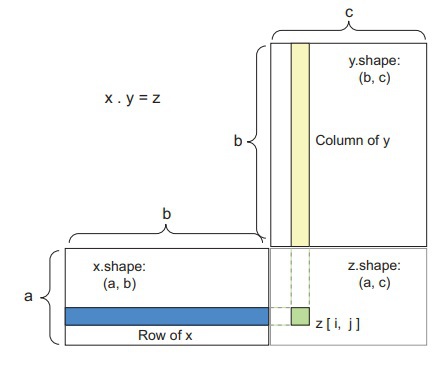
The shape compatibility between tensors for dot product operations can be very confusing and misleading at times. Below is a box diagram that is aimed at improving the reader’s visualization of the input and output tensors.
In this diagram, the tensors x, y, and z have been depicted as rectangles. For a dot product, the rows of the tensor “x” must be matching in size with the columns of the tensor “y,” hence this would insinuate that in the above box diagram, the width of the “x” rectangle should match the height of the “y” rectangle.
In the case of tensors that are of higher-dimensions, the dot product between these tensors would follow the shape compatibility rules as in the case for 2D tensors:
(a, b, c, d) . (d,) -> (a, b, c)
(a, b, c, d) . (d, e) -> (a, b, c, e)
Tensor Reshaping
The third tensor operation which we will be discussing is the tensor reshaping. We did not use tensor reshaping in the example of the Neural network, which was using dense layers. However, the tensor reshaping operation was used for preprocessing data pertaining to the digits prior to giving it to the Neural network, this example was:
train_images = train_images.reshape((60000, 28 * 28))
The term reshaping is self-explanatory. The tensor on which this operation is applied is basically reshaped (basically rearrangement of the rows and columns) to match the desired shape, which is detailed beside the operation. Furthermore, it is important to keep in mind that tensor reshaping only rearranges the rows and columns, not change them. Hence, the total number of coefficients (of the original tensor) remains the same for the reshaped tensor. Here’s a simple example to better understand reshaping:
>>> x = np.array([[0., 1.],
[2., 3.],
[4., 5.]])
>>> print(x.shape)
(3, 2)
>>> x = x.reshape((6, 1))
>>> x
array([[ 0.],
[ 1.],
[ 2.],
[ 3.],
[ 4.],
[ 5.]])
>>> x = x.reshape((2, 3))
>>> x
array([[ 0., 1., 2.],
[ 3., 4., 5.]])
Aside from simply rearranging the rows and columns of a tensor in reshaping, another type of reshaping is also very common, known as transposition. Unlike reshaping where the shape of a tensor is changed by rearrangement, transposition basically exchanges the position of the rows with the columns, hence turning rows into columns and columns into rows. In transposition, a tensor
y[j, :] becomes
y[:, j]
>>> x = np.zeros((150, 10))
>>> x = np.transpose(x)
>>> print(x.shape)
(10, 150)
Gradient-Based Optimization in Neural Networks
In the preceding sections, specifically in the element-wise operation section, the data inputted in a Neural network is transformed by each layer of the network as shown below:
output = relu(dot(W, input) + b)
We will now analyze the elements of this expression. Two attributes are very interesting. These attributes are “W” and “b” respectively. They are known as the “weight” and “trainable parameters” of any layer, and in more technical terms, they are referred to as the kernel
and bias
attributes of a layer, respectively. The weights essentially store the data, which is learned by the system during training.
In the beginning, the weight matrices are observed to have a bunch of random values filling them. These random values are generated through a step known as random initialization. Although the above expression will not yield any useful results as the parameters of the attributes generated are random. However, everything needs to have a starting point, and for machine learning, this is the starting point because of the fact that the system will respond to the feedback signal and adjust these weights accordingly. Hence, we have now discussed what training is, the gradual adjustment of weights according to a feedback signal is called training, and this is the essence of machine learning.
The training of a network is done in training loops
. The following steps outlined below explain a typical training loop routine, and they are repeated as long as necessary:
- Take a collection of training samples labeled “x” along with the corresponding targets of these samples labeled “y.”
- This step is known as the forward pass
. Once the batch of the samples and targets have been drawn, proceed to get the predictions y_pred
by running the Neural network on the training sample “x.”
- Measure the results with the prediction and note any mismatch and discrepancies between the two values. This is basically computing the loss of the network.
- Update the weights of the Neural network. Keep in mind that the weights should be updated in a way to lower the loss on this collection or batch.
Through this training loop, we will eventually obtain a network that exhibits considerably low levels of discrepancies and mismatching between the predictions and targets, i.e., a mismatch between y_pred and y, respectively. Hence, the network has essentially learned how to map the data inputs to the corresponding correct targets correctly.