Chapter 3: Starting Our Tasks with Neural Networks
In this chapter, we will discuss the practical applications of Neural networks in more detail and incorporate the concepts we went through in the previous chapters. Moreover, the main focus of this chapter will be a chance for the reader to reinforce his knowledge of deep learning and neural network while going through problems that address the most common practical uses of Neural networks which are:
- Binary classification
- Multiclass classification
- Scalar regression
In addition, this chapter will give an introduction to the deep learning libraries we will be using throughout this book, namely the Python and Keras deep learning libraries. The topics will include a closer and detailed inspection of some of the core components discussed in the previous chapter such as:
- Layers, networks, objective functions and optimizers
Before we proceed with the chapter, here are the practical examples which we will be a demonstration on how we can use Neural networks to solve real-world issues:
- Identifying if the movie reviews are either positive or negative (Category: of binary classification)
- Cataloging the new wires according to the topic (Category: Multiclass classification)
- By inputting real-estate data to the network, we procure price estimations for houses (Category: Scalar regression)
After concluding this chapter, the reader will be able to make use of Neural networks and implement it to solve machine problems of simple nature; for instance, the classification and regression over vector data.
Inspection of a Neural Network
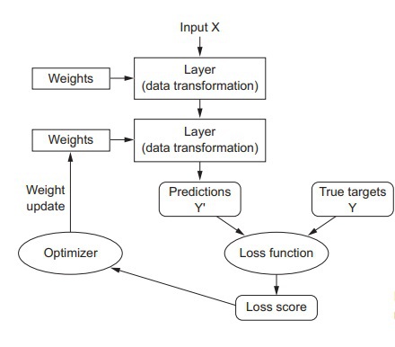
From our preceding discussions we have concluded that the Neural network’s training essentially depends upon the following objects:
- Layers that have been merged together forming a network (or in other words, a model)
- The data which has been inputted into the Neural network and the targets which correspond to this input data
- The loss function (this function essentially the defining factor for the feedback signal that is purposed for learning)
- The optimizer (the determinant of the learning procedure)
Below is a figure which emphasizes the relationship between these objects (the network, the layers, the loss function, and the optimizer):
Before moving further, let’s discuss these anatomical elements of a Neural network in more detail.
Layers
By now, we have become familiar with the importance of layers as the building blocks of deep learning. To reiterate the concept in brief and simple terms, a data-processing module that receives an input in the form of a tensor (can be one or two tensors) and gives an output in the form of a tensor as well can be one or two tensors) is known as a layer. In addition to this, we discussed the attributes of a layer, such as the “weight briefly.” The weight of a layer refers to its state. While some layers may be stateless, most of the layers possess a state (several tensors that are learned with stochastic gradient descent, these tensors as a group form what we term as, the network’s knowledge
).
Aside from this, different types of layers are suitable for different purposes (different tensor formats and different types of data processing needs). The types of layers we have discussed so far include:
- Densely connected layers
- Recurrent layers
- Convolution layers
To elaborate further, we can consider an example of a simple vector data which is contained within a 2D tensor of shape (samples, features
). Dense layers will process such a tensor. Similarly, a 3D tensor with a shape of (samples, timestamps, features
) storing a type of data known as a “sequence data,” will be processed by a recurrent layer (for instance, an LTSM layer). Furthermore, if we are dealing with image data, then the corresponding container will be a 4D tensor, and such a tensor is typically processed by a layer known as CONV2D, which is basically a 2D convolution layer.
In the Keras framework, building a deep-learning model is just like joining pieces of a puzzle together. To be more specific, deep-learning models are built upon data-transformation pipelines that are actually made by putting together compatible layers. In this context, compatibility refers to the ability of a specific type of layer to be able to accept tensors that have a specific shape as input and return corresponding tensors of a specific shape. For example:
from keras import layers
layer = layers.Dense(32, input_shape=(770,))
In this example, we have created a dense layer that is specified only to accept 2D tensor inputs in which the very first dimension is 770. Moreover, we have left the batch dimension as unspecified and because of this the layer will accept any value. Hence, the input tensor will be a 2D tensor with a shape of (770,) and the output tensor will have its first dimension changed to 32. Meaning that the layer we have built above is only able to be connected to a downstream layer, which is specified to accept vector inputs that are 32 dimensional. In Keras, the hassle of considering each layer’s compatibility becomes non-existent because of the fact that each layer added to the model is built dynamically so that it can match with the shape of the next layer. For example, we have added another layer on top of an existing one while using Keras:
from keras import models
from keras import layers
model = models.Sequential()
model.add(layers.Dense(32, input_shape=(770,)))
model.add(layers.Dense(32))
We can see that the layer succeeding the last one is devoid of any input shape argument. Regardless of not receiving an input shape argument, the second layer has inferred that its input shape should be the output shape of the preceding layer.
Models
Deep learning models are essentially a network of layers directed into an acyclic graphical form. The simplest form of a deep learning model would be one that is made up of a linear network of layers. Such a model is capable of only single mapping tensors, i.e., one input to one corresponding output.
However, as we progress further understanding the anatomical features of Neural networks, we come to know that there is a large variety of topologies for Neural networks, which in turn, form a variety of deep learning models. Following are the most common:
- Two-branch networks
- Multihead networks
- Inception blocks
Now let’s elaborate on the concept of Neural network topologies. Basically, a Neural network works in a pre-defined space of possibilities, and it is within this space that the network looks for viable representations of data. Hence, a topology essentially defines a constrained and pre-defined space for a Neural network, and because of this, a Neural network topology is also termed as a “hypothesis space.” Hence, selecting a specific topology will essentially limit the network’s hypothesis space to only a particular set of tensor operations. Hence, the main focus of your job would be to simply look for the optimal set of values for the specific topology’s corresponding weight tensors.
As such, selecting the most optimal network architecture for your deep learning model is closer to being an artistic choice rather than a logically sound decision. This is because no defined parameter dictates whether a network topology is superior to the other or if it is the right one for your model. This is why a good neural-network architect can only develop a good intuition for choosing network architectures through repeated practice.
Loss Functions and Optimizers
Now, after deciding on network architecture and successfully defining it for the deep learning model, there are still two things that are missing and require our immediate attention, namely:
- The Loss Function: also known as the objective function. This represents the minimized quantity in the training session of a model. In other words, the success rate of the task which the network is working on.
- Optimizer: It works according to the results of the loss function in the sense that the Neural network’s data update is done according to the loss function, hence controlled by the optimizer. The optimizer uses an implementation of a variant of an SGD (stochastic gradient descent).
One interesting point to note about the loss functions and the gradient descent process is that within a Neural network that is architecture as a multi loss network, there can be multiple loss functions to accommodate the multiple outputs of the network. However, the same thing does not apply to a gradient descent process. Instead, the gradient descent process is always based upon one singular scalar loss value, therefore in multi loss networks, a technique known as “averaging” is used to merge the multiple losses into a singular scalar value.
A very important point to always keep in mind when working with Neural networks is always to try to select the most optimal and correct objective function for a given problem. The reason for this is because a Neural network will always look for shortcuts and choose that path to keep the loss at a minimum. Hence, if we do not make sure of the clarity of the objective and its correlation to the success of the given task, the Neural network will perform actions that are either unnecessary or unwanted. So choosing a correct objective will save one from facing these unpredictable side-effects.
What is Keras?
In the previous sections of this book, we have studied demonstrations and examples of code that are using Keras. In this section, we will discuss what Keras actually is in detail. To define Keras, it is simply a framework for Python, which is specialized for deep-learning projects. Due to this, Keras provides programmers with a simple and convenient route towards being able to define and train deep-learning models of almost any kind. Although this framework was originally developed for people that were researchers to facilitate them with fast-experimentation, its functionality made it suitable for being used in deep-learning models as well.
The core features of the Keras framework include:
- Allows code to be cross-run between the GPU and CPU. Meaning that the source code is compatible with both of the components without needing to make any changes to it.
- By featuring a user-friendly API, Keras makes it easier for users to prototype deep-learning models with incredible convenience.
- Keras also conveniently features native support for both convolutional and recurrent networks or any combination of these two types of networks. By having built-in support for these networks, Keras indirectly provides native support for computer vision and sequence processing.
- The reason why Keras can be used for almost any type of Neural network is because it supports arbitrary network architectures. In other words, if you are looking to build a generative adversarial network to even a Turing machine, Keras remains relevant and appropriate for the task.
Keras and the Backend Engines
A distinctive feature of Keras is that being a model-level library in Python, it is associated with the supply of high-level basic elements and operations to develop a deep learning model. On the other hand, Keras does not associate itself with low tier operations (for example, tensor manipulation and differentiation). To make up for this, Keras includes a well-optimized tensor library specialized just for this purpose, and such libraries serve the purpose of being the backend engines of Keras. Moreover, Keras does not include a single exclusive backend engine. Instead, Keras supports multiple different backend engines with seamless support. Following are the three most popular backend engines supported by Keras:
- TensorFlow backend
- Theano backend
- Microsoft Cognitive Toolkit (CTNK) backend
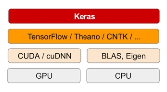
The modular architecture of Keras is shown in a visual representation below:
In addition, the code written on Keras is capable of being executed by these backends without any changes made to the source code, and the different backends can be swapped out if a specific backend proves to be more efficient and faster for a specific task. The TensorFlow backend enables the Keras framework to run on both CPUs and GPUs efficiently. This is possible as TensorFlow uses further smaller libraries as its own backend, and these backends are different for when running code on a CPU and for a GPU. For a CPU, TensorFlow uses a low tier library known as “Eigen” for performing tensor operations. At the same time, in a GPU, TensorFlow utilizes the popular cuDNN (Nvidia Cuda Deep Neural Network) library developed and optimized by NVIDIA.
A Short Overview of Deep Learning Development with Keras
If we look back, we will see that in the MNIST example demonstrated in the early chapters of this book, are also an example of a Keras model. Keeping this example in mind, a standard Keras workflow is exactly the same as shown in that demonstration. Here’s a quick and brief overview of the elements of a Keras workflow:
- Specifying the input tensors and the corresponding target tensors (collectively known as the training data).
- Build a deep learning model that optimally maps the input tensors to the target tensors. Remember that a model is just a combination of layers in a network.
- Select the elements (loss function, optimizer, and metrics to monitor) through which the network’s process of learning can be configured and customized.
- Keep repeating the fit() method of the deep learning model on the training data.
A deep learning model can be defined and specified by using either of the two methods (depending on how many layers a model has):
- Using the Sequential class. This method is viable only for models that are built up from linear stacks of layers.
- Using the functional API. This method is viable for models that are made up of an acyclic graph of layers supporting arbitrary model architectures.
To refresh our memory, below is an example of a model being defined by the Sequential class. Note that the deep learning model has a linear stack of two layers:
from keras import models
from keras import layers
model = models.Sequential()
model.add(layers.Dense(32, activation='relu', input_shape=(770,)))
model.add(layers.Dense(10, activation='softmax'))
Similarly, an example is shown below that shows a deep learning model being defined by a functional API:
input_tensor = layers.Input(shape=(770,))
x = layers.Dense(32, activation='relu')(input_tensor)
output_tensor = layers.Dense(10, activation='softmax')(x)
model = models.Model(inputs=input_tensor, outputs=output_tensor)
If we examine this demonstration, then we can see that the functional API is essentially concerned with manipulating the data tensors. Now, these data tensors are the ones that the deep learning model processes, and as such, the functional API manipulates them and applies layers to these tensors, treating them as functions rather than tensors.
Once we have specified and defined the architecture of our deep learning model, the notion of having used either the sequential class or the functional API no longer holds any importance. This is due to the reason that the steps which come after this will be the same regardless of the method used for defining the model.
In the compilation step, we proceed to choose the loss function and optimizer and hence, configuring the learning process of the deep learning model. In addition, we can also select some metrics that we want to monitor in the training session of the model. Now let’s see a simple and common example of a model in the compilation step being specified one loss function:
from keras import optimizers
model.compile(optimizer=optimizers.RMSprop(lr=0.001),
loss='mse',
metrics=['accuracy'])
Now, the last thing left to do is using the fit() method to pass the NumPy arrays of training data (the input data and the corresponding target data) to the deep learning model, as shown below:
model.fit(input_tensor, target_tensor, batch_size=128, epochs=10)
The Pre-requisites for a Deep Learning Workstation
In this section, we will discuss what you need to set up your deep learning workstation. We will look at what is necessary, what is optional and what can speed up your work and what can slow it down, all of the aspects you would want to know about when putting together your workstation for deep learning.
The first point of discussion is the importance of a GPU in a deep learning workstation. While you may think that a deep learning code run on multicore and fast CPU seems adequate, that is not the case. A GPU is highly recommended for running deep learning code because it not only increases the speed factor by a whopping five or even 10. Moreover, deep learning code for applications, such as image processing (made up of a convolutional Neural network,) will be immensely slow and time-consuming. In such cases, a GPU proves to be the ideal contender as it not only increases the speed of the entire work process, but modern NVIDIA GPUs also feature well-optimized and dedicated “Tensor” cores developed for such tasks. In short, using a NIVIDA GPU is highly recommended for your deep learning workstation. Although there are cloud solutions, such as Google’s cloud platform, it can prove to be very expensive and inefficient in the long run.
Furthermore, the recommended operating system for a deep learning workstation, regardless of the GPU you are using (Nvidia or a Cloud solution), the recommended OS is Unix. Although the Keras backends do support Windows, it is still desirable if you choose Unix, or just install an Ubuntu OS as a dual boot alongside the Windows OS in your machine - Ubuntu will save a huge chunk of your time and resource later as compared to Windows so keep this in mind. In addition, before you can use Keras, you will also need to install its backend engines, i.e., TensorFlow, Theano, CNTK, or even all of them (if you intend to switch between the backend engines more often). However, be mindful that this book will focus primarily on TensorFlow and occasionally discuss Theano; however, we will discuss CNTK.
If you have the budget, go for the latest Nvidia Quadro GPUs as they have the most vRAM in the current GPU industry and dedicated tensor cores for such experiments. Moreover, Nvidia is the only company that has heavily invested in the deep learning market, hence the support and compatibility it provides for deep learning projects are outstanding and the best at the moment.
Jupyter Notebooks
Arguably the most efficient way to run any deep learning experiment is by using a Jupyter notebook. The Jupyter notebook is an application that generates a file known as a “notebook.” This file can easily be edited in the browser, giving the best of both worlds, being able to execute Python code while also having the ability to annotate (what you are doing in) the code with rich text-editing features of the Jupyter notebook. This is why Jupyter Notebooks is so popular among the communities of data science and machine learning niche.
You can easily turn long experiments into smaller components with the ability to execute each small component independently, meaning that if you come across a problem in the later parts of your code, you can just execute the smaller components to find where the problem is instead of executing the entire code from the beginning to the end.
Jupyter Notebooks is not a necessary requirement for setting up your deep learning workstation as you can just execute the deep learning code from the standalone Python scripts within the IDE. Still, it is recommended to use this application for the sake of your convenience.
Deep Learning Binary Classification Example
We will now discuss the examples which we briefly discussed in the introduction of this chapter. The first example will be a machine learning problem that is most common in the real world, binary classification. The situation we will consider for the demonstration is that we need to set up a deep learning model to classify movie reviews as either positive or negative by giving it input data of the text content of the reviews being classified.
Dataset to be Used
The dataset we will be using for our deep learning model is the Internet Movie Database (IMDB), which consists of a set of fifty thousand (50,000) reviews that are highly polarized. Moreover, this set of reviews is split into two equal parts. One part consists of 25,000 reviews for training the deep learning Neural network and the other part consists of 25,000 reviews for testing the deep learning network; each of these parts has a percentage of 50% negative and 50% positive reviews.
The reason we always use a separate test for testing the deep learning model is that using the same set it has been trained on is practically useless as the machine, as well as the user already knows the labels of the training set. Moreover, our main concern is to use this deep learning model for helping us with data that neither the machine has seen nor the user has sorted before.
Similar to when we used the MNIST dataset, it came preloaded with the Keras framework. The IMDB dataset also comes packaged with the same Keras framework. Hence we do not need to load it up separately. Moreover, the IMBD dataset already has preprocessed data, i.e., the sequence of words in the reviews has already been transformed into the corresponding sequence of integers (each of these integers corresponds to a word in the system’s defined dictionary).
We will now proceed to load the IMDB dataset into our workstation. To do this, we will use the following lines of code:
from keras.datasets import imdb
(train_data, train_labels), (test_data, test_labels) = imdb.load_data(
num_words=10000)
If you look at the above lines of code, you’ll see that there is an argument num_words=10000
. This argument tells the system only to retain 10000 words that are the most frequently occurring in the dataset. By doing this, we discard the rare words used in the dataset and keep the size of vector data within a manageable range.
In the dataset, the labels (train_labels and test_labels) are basically the preprocessed integers 0 and 1 that indicate the corresponding annotation of the words. A word with a label integer “0” is a word with negative annotation, and a word with a label integer “1” is a word with positive annotation.
>>> train_data[0]
[1, 14, 22, 16, ... 178, 32]
>>> train_labels[0]
1
As we have already restricted the system to the top 10,000 most frequently used words, hence it is a given that no word index will exceed past this limit.
>>> max([max(sequence) for sequence in train_data])
9999
To decode the preprocessed reviews back into English, use the following lines of code (this is just for informative purposes, it’s not necessary to perform this step in the usual sequence of things):
word_index = imdb.get_word_index()
reverse_word_index = dict(
[(value, key) for (key, value) in word_index.items()])
decoded_review = ' '.join(
[reverse_word_index.get(i - 3, '?') for i in train_data[0]])
In the first line, the argument word_index is the dictionary responsible for mapping the corresponding words to integers.
Preparing to Feed Data into the Neural Network
The data we have so far is still not ready to be fed into the Neural network yet. What we have is data in the form of integers, and what we need is data in the form of tensors. Hence the next plan of action is to convert this list of integers into tensors. This can be done in two ways which are:
- First, we convert the data lists such that all of the lists are of the same length. This is done by padding them. After this, we proceed to convert the same length integer lists into integer tensors. Be mindful that the shape of these tensors should be (samples, word_indices). We will now use the embedding layer as the first layer in the Neural network because it can handle these integer tensors.
- The second method is to turn the data lists which we are working with into vectors. These vectors would be 0s and 1s, and this conversion can is done by one-hot encoding the data lists. The practical meaning of what this insinuates is that a sequence let's say [2, 4] is converted into a vector that is 10,000 dimensional. This vector would be largely 0s, with the exception of the two indices, 2 and 4. These indices would be vector 1s, and the rest of the indices would be vector 0s. To handle such type of floating data, we will use a dense layer as the first layer in the Neural network.
In this example, we will use the second method to convert the list of integers into tensors (vectorizing the source data). This will be done manually as follows:
import numpy as np
def vectorize_sequences(sequences, dimension=10000):
results = np.zeros((len(sequences), dimension))
for i, sequence in enumerate(sequences):
results[i, sequence] = 1.
return results
x_train = vectorize_sequences(train_data)
x_test = vectorize_sequences(test_data)
After performing this step, the data samples would now look like this:
>>> x_train[0]
array([ 0., 1., 1., ..., 0., 0., 0.])
Apart from vectorizing the train_data and test_data, we should also vectorize the train_labels and test_labels. This is not hard, on the contrary, it is actually pretty straightforward as you can see from the two lines of code below:
y_train = np.asarray(train_labels).astype('float32')
y_test = np.asarray(test_labels).astype('float32')
Now, our data is ready to be inputted into the Neural network of the deep learning model.
Establishing the Neural Network
Here’s a summary of the ingredients we are working with so far to build our Neural network. Our training data is made up of vectors (the input data) and scalars (the labels).
Now, we have to choose a type of network that works best with our ingredients, and so far, the choice is very straightforward and simple because we know that with such type of data, a dense
layer will work best. Hence, our Neural network will be one that has completely connected stacks of layers featuring relu
activations. Hence the argument to define such a network would be:
Dense(16, activation='relu').
The above argument is specifying the number of hidden units (16) of layers that are to be passed to each dense layer. To refresh our memory below is the chain of tensor operation that is typically implemented by a dense layer with a relu activation:
output = relu(dot(W, input) + b)
Since we have a total of 16 hidden units, the above matrix W (also known as the weight matrix) will be shaped as (input_dimension, 16).
Similarly, if we consider a dot product of this weight matrix W, the input data will end up being projected onto representation space that is actually 16-dimension.
It is also important to understand the meaning of a representation’s space dimensionality. In essence, the dimensionality of a representation space defines the freedom with which you allow the Neural network to learn internal representations. So, if we have a greater number of hidden units, this means that we are allowing for a bigger high-dimensional space of representation. Thus, the Neural network has more freedom in regards to being able to learn representations that are even more complex; however, with more freedom to learn comes greater risks. It becomes harder to control what the network learns, and may lead to the Neural network learning patterns that are useless or may even harm the success potential, so be wise when making such a network.
Regarding the network architecture, you should always ask yourself these two questions when implementing a stack of dense layers into the Neural network:
- How many layers should I use?
- What’s the optimal number of hidden units that I should appoint to each layer?
In this example, we sought the following answers to the questions above:
- About two intermediate layers, each having a total of 16 hidden units.
- A third layer, whose job will be to take the scalar predictions as its output. The prediction will be the annotation of the current review being analyzed (if the review is positive or negative).
In addition, the activation functions for the intermediate and third (final) layer are also different. The intermediate layer uses relu
as the activation function while the third layer is using the sigmoid as the activation function. This is down to the nature of its job (outputting a probability value of either 0 or 1, for instance, a probability value of 1 depicts the likelihood of a review of being positive and vice versa).
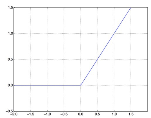
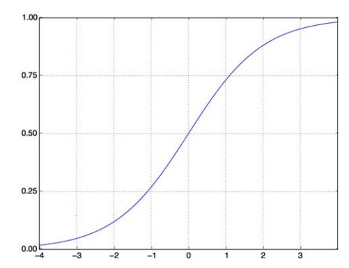
The job of the relu function is to take the negative values and convert them into zeroes. On the other hand, a sigmoid function basically forces all arbitrary values into an interval of the shape [0, 1], giving us an output which can then be interpreted as a probability.
A Rectified Linear Unit Function (relu)
A Sigmoid Function
The Keras implementation of the building this network is shown below:
from keras import models
from keras import layers
model = models.Sequential()
model.add(layers.Dense(16, activation='relu', input_shape=(10000,)))
model.add(layers.Dense(16, activation='relu'))
model.add(layers.Dense(1, activation='sigmoid'))
The final step to complete the Neural network is to select a suitable loss function and an optimizer. Before making your choice, analyze the network you have built so far and ponder on what type of loss function would be the most optimal considering the type of problem we are tackling. In this case, as we are dealing with a problem relating to binary classification and the output of our network is in the form of a probability value, then the ideal choice would be to go for a binary_crossentropy
loss function. While there are other choices available such as the mean_squred_error
loss function, we will still go for the former as we are working with a network that gives an output of probability values. Cross-entropy is the most suitable for such situations. The reason why cross-entropy is a good contender is because of its function - it basically measures the distance between the probability distributions and the predictions.
So we are going with the cross-entropy loss function, and the optimizer we are choosing is the rmsprop
optimizer. The metric which we will monitor during the training is the “accuracy.” To implement these elements into the network, we will use the following lines of code:
model.compile(optimizer='rmsprop',
loss='binary_crossentropy',
metrics=['accuracy'])
We can pass off these elements as strings due to the fact all of them (binary_crossentropy, rmsprop, and accuracy) are basically part of the Keras framework.
We can also configure our optimizer (its parameters) according to our needs by simply passing the optimizer class as an argument. Pretty simple as shown below:
from keras import optimizers
model.compile(optimizer=optimizers.RMSprop(lr=0.001),
loss='binary_crossentropy',
metrics=['accuracy'])
We can also use custom loss functions and metrics as shown below:
from keras import losses
from keras import metrics
model.compile(optimizer=optimizers.RMSprop(lr=0.001),
loss=losses.binary_crossentropy,
metrics=[metrics.binary_accuracy])
Validating the Approach
To monitor the accuracy of the deep learning model during its training, we need to create a “validation set” by setting aside a portion of samples from the training dataset. Let’s set aside 10,000 samples for our validation dataset as shown below:
x_val = x_train[:10000]
partial_x_train = x_train[10000:]
y_val = y_train[:10000]
partial_y_train = y_train[10000:]
Repeating the training process for a dataset is known as an epoch. Once we have created a validation set, we will proceed with training the deep learning model for a total of 15 epochs on the samples x_train and y_train. This training will be done in batches with a size of 256 samples per batch. Moreover, the accuracy and loss of the samples we previously set aside (the 10,000 samples) will also be monitored. To do this, we will simply pass the set as an argument, i.e., validation_data as shown below:
model.compile(optimizer='rmsprop',
loss='binary_crossentropy',
metrics=['acc'])
history = model.fit(partial_x_train,
partial_y_train,
epochs=15,
batch_size=256,
validation_data=(x_val, y_val))
It takes for an epoch to complete on a CPU is roughly 2 seconds or even less than 2 seconds. The entire process of training is completed in a timeframe of 15 seconds, and when an epoch is completed, there is a brief pause before the next epoch starts. This pause happens so that the model can easily compute the loss and accuracy (in our case, it is computed on the validation dataset, which consists of ten thousand samples).
One more noticeable aspect of the model’s working is that when we use the function model.fit(), we get a history
object. The specialty of this “history” object is that it holds the data pertaining to everything that happened in the training process in the form of a dictionary.
>>> history_dict = history.history
>>> history_dict.keys()
[u'acc', u'loss', u'val_acc', u'val_loss']
Upon further analysis, we come to know that there are four distinct entries within the dictionary, and each entry is a per metric record of their values in the training session and validation session. We will now proceed to use the Matplotlib library to plot the losses and accuracy of both training and validation datasets beside each other.
import matplotlib.pyplot as plt
history_dict = history.history
loss_values = history_dict['loss']
val_loss_values = history_dict['val_loss']
epochs = range(1, len(acc) + 1)
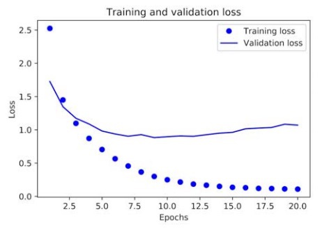
plt.plot(epochs, loss_values, 'bo', label='Training loss')
plt.plot(epochs, val_loss_values, 'b', label='Validation loss')
plt.title('Training and validation loss')
plt.xlabel('Epochs')
plt.ylabel('Loss')
plt.legend()
plt.show()
In the above demonstration, the label “bo” basically refers to a blue dot in the resulting graphical representation, and the label “b” refers to a static blue line in the same graph as shown below:
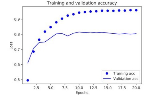
Now for plotting the accuracy of the training and validation datasets:
plt.clf() ‘clearing the figure’
acc_values = history_dict['acc']
val_acc_values = history_dict['val_acc']
plt.plot(epochs, acc, 'bo', label='Training acc')
plt.plot(epochs, val_acc, 'b', label='Validation acc')
plt.title('Training and validation accuracy')
plt.xlabel('Epochs')
plt.ylabel('Loss')
plt.legend()
plt.show()
From these two graphs, we can clearly see the trend that with every training epoch, there is a visible decrease in loss and an increase in accuracy as we move through epochs. This is the essence of gradient descent optimization, which basically decreases the quantity which we want to minimize every epoch or iteration. However, the trend seems to take the opposite turn in the cases of validation loss and accuracy.
Both the loss and accuracy are seen to peak out at the 4th
epoch. This is an accurate representation of the warnings given to learning programmers that a deep learning model performing outstandingly on a training dataset is not sure to have to the same success on a new dataset, such as the validation dataset in our case. The exact phenomenon that we are dealing with is basically “overfitting,” in other words, the training has become over-optimized, and the representations being learned by the model are too specific. Hence, there is no generalization to account for data that is outside the training dataset.
There is a range of techniques through which overfitting can be mitigated, which we will discuss in the coming chapters. For now, we could tackle the issue of overfitting by just stopping the training session just before it peaks, i.e., after three epochs.
Now let’s train a new Neural network for four epochs and observe the results when testing it on new data:
model = models.Sequential()
model.add(layers.Dense(16, activation='relu', input_shape=(10000,)))
model.add(layers.Dense(16, activation='relu'))
model.add(layers.Dense(1, activation='sigmoid'))
model.compile(optimizer='rmsprop',
loss='binary_crossentropy',
metrics=['accuracy'])
model.fit(x_train, y_train, epochs=4, batch_size=256)
results = model.evaluate(x_test, y_test)
The end results are as shown below:
>>> results
[0.2929924130630493, 0.88327999999999995]
With such an ordinary approach, we scored an accuracy of 88%. Hence, if we use top of the line approaches, scoring accuracy of 95% would be fairly easy.
Using this Trained Network for New Data
After we have trained the Neural network, we can now use it for our own practical purposes, which was to classify the reviews as positive or negative. To do this, we will be using the predict
method as shown below:
>>> model.predict(x_test)
array([[ 0.98006207]
[ 0.99758697]
[ 0.99975556]
...,
[ 0.82167041]
[ 0.02885115]
[ 0.65371346]], dtype=float32)
This shows the predictive results of the likelihood of a review to be positive or negative.
We cannot go into the very fundamental details of the following examples, as you should already have an idea of what’s happening in the lines of code. We will be giving brief explanations and go through these examples to save our resources for more important discussions in the following chapters.
Deep Learning Multiclass Classification Example
In this example, the task faced by the Neural network will be to classify the newswires of Reuter into 46 mutually exclusive topics. The classes in this example are 46, making it a multiclass classification problem, more specifically a single-label multiclass classification problem because each class is exclusive from one another.
The Reuters Dataset
For this example, we will be working with the Reuters dataset. It comes preloaded with the Keras library, so it is easy to use as shown below:
from keras.datasets import reuters
(train_data, train_labels), (test_data, test_labels) = reuters.load_data(
num_words=10000)
The number for samples for train_data and test_data are as follows:
>>> len(train_data)
8982
>>> len(test_data)
2246
The word indices are in the form of a list of integers, just like the IMDB reviews in the previous example.
>>> train_data[10]
[1, 245, 273, 207, 156, 53, 74, 160, 26, 14, 46, 296, 26, 39, 74, 2979,
3554, 14, 46, 4689, 4329, 86, 61, 3499, 4795, 14, 61, 451, 4329, 17, 12]
These list of integers can be decoded as follows:
word_index = reuters.get_word_index()
reverse_word_index = dict([(value, key) for (key, value) in word_index.items()])
decoded_newswire = ' '.join([reverse_word_index.get(i - 3, '?') for i in
train_data[0]])
Preparing the Data
We will now proceed to vectorize the data by using the same code we outlined in the previous example:
import numpy as np
def vectorize_sequences(sequences, dimension=10000):
results = np.zeros((len(sequences), dimension))
for i, sequence in enumerate(sequences):
results[i, sequence] = 1.
return results
x_train = vectorize_sequences(train_data)
x_test = vectorize_sequences(test_data)
As discussed earlier, data can be vectorized either by label listing it as an integer tensor or by one-hot encoding (mainly used for categorical encoding). The method of one-hot encoding is shown below:
def to_one_hot(labels, dimension=46):
results = np.zeros((len(labels), dimension))
for i, label in enumerate(labels):
results[i, label] = 1.
return results
one_hot_train_labels = to_one_hot(train_labels)
one_hot_test_labels = to_one_hot(test_labels)
This can also be done natively in Keras, as we did in the MNIST example in the beginning:
from keras.utils.np_utils import to_categorical
one_hot_train_labels = to_categorical(train_labels)
one_hot_test_labels = to_categorical(test_labels)
Building the Neural Network
This case is similar to the binary classification problem; however, the methods and parameters used will be completely different because adopting the same procedure, and choosing the same attributes would lead to big information bottlenecks.
For this scenario, we will be using a larger layer with 64 unit
from keras import models
from keras import layers
model = models.Sequential()
model.add(layers.Dense(64, activation='relu', input_shape=(10000,)))
model.add(layers.Dense(64, activation='relu'))
model.add(layers.Dense(46, activation='softmax'))
Since the output of the layers is in the form of a probability, hence we will be using the categorical_crossentropy
as our loss function. We can improve the result by minimizing the distance between the probability distribution output of the network and the true distribution of the labels.
model.compile(optimizer='rmsprop',
loss='categorical_crossentropy',
metrics=['accuracy'])
Validating the Approach
The validation dataset for this network will consist of 1,000 samples.
x_val = x_train[:1000]
partial_x_train = x_train[1000:]
y_val = one_hot_train_labels[:1000]
partial_y_train = one_hot_train_labels[1000:]
We will train the network for 15 epochs (be mindful that the graphical representation will show upto 20 epochs so don’t be bothered by that):
history = model.fit(partial_x_train,
partial_y_train,
epochs=15,
batch_size=512,
validation_data=(x_val, y_val))
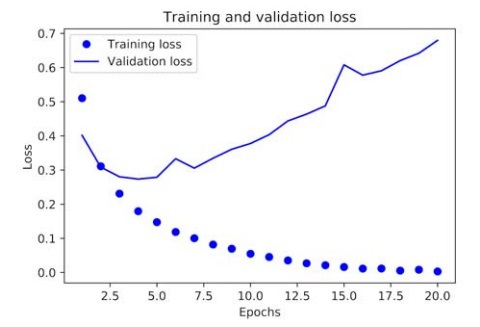
We will now move towards showcasing the graphical representation of the loss and accuracy metrics.
For the loss of the training and validation sets:
import matplotlib.pyplot as plt
loss = history.history['loss']
val_loss = history.history['val_loss']
epochs = range(1, len(loss) + 1)
plt.plot(epochs, loss, 'bo', label='Training loss')
plt.plot(epochs, val_loss, 'b', label='Validation loss')
plt.title('Training and validation loss')
plt.xlabel('Epochs')
plt.ylabel('Loss')
plt.legend()
plt.show()
For the accuracy of the training and validation sets:
plt.clf()
acc = history.history['acc']
val_acc = history.history['val_acc']
plt.plot(epochs, acc, 'bo', label='Training acc')
plt.plot(epochs, val_acc, 'b', label='Validation acc')
plt.title('Training and validation accuracy')
plt.xlabel('Epochs')
plt.ylabel('Loss')
plt.legend()
plt.show()
From the graphical representation, we can see that the overfitting phenomenon comes into play after 9 epochs. So we will train a new network for only 9 epochs and then test it on the testing dataset:
model = models.Sequential()
model.add(layers.Dense(64, activation='relu', input_shape=(10000,)))
model.add(layers.Dense(64, activation='relu'))
model.add(layers.Dense(46, activation='softmax'))
model.compile(optimizer='rmsprop',
loss='categorical_crossentropy',
metrics=['accuracy'])
model.fit(partial_x_train,
partial_y_train,
epochs=9,
batch_size=512,
validation_data=(x_val, y_val))
results = model.evaluate(x_test, one_hot_test_labels)
After training, the results we obtain are shown below:
>>> results
[0.9565213431445807, 0.79697239536954589]
We obtain an accuracy of approximately 80% by using this approach. When compared to a random baseline, these results are good. The results shown by a random baseline would be as follows:
>>> import copy
>>> test_labels_copy = copy.copy(test_labels)
>>> np.random.shuffle(test_labels_copy)
>>> hits_array = np.array(test_labels) == np.array(test_labels_copy)
>>> float(np.sum(hits_array)) / len(test_labels)
0.18655387355298308
Hence, 19% would be the accuracy.
Generating Predictions on New Data
We will now take all of the data from the testing set and generate topic predictions for it. Each entry in the predictions
method will be a 46 length vector with coefficients summing to 1 along with the last line of code showcasing the class with the highest probability:
predictions = model.predict(x_test)
>>> predictions[0].shape
(46)
>>> np.sum(predictions[0])
1.0
>>> np.argmax(predictions[0])
4
Deep Learning Regression Example
In the previous examples, we dealt with problems relating to binary classification and multiclass classification, which was solved by training a Neural network such that when it would be given an input data point, it would be able to predict its discrete label.
This example relates to an entirely different machine learning problem known as regression. Instead of predicting a discrete label, the Neural network is required to predict a continuous value (for instance, meteorological predictions).
This example will focus on predicting house prices.
The Boston Housing Price Dataset
The dataset we will be using is the Boston Housing Price dataset, which features data points of the Boston suburb in the era of the mid-1970s. The goal is to predict the median house prices while taking into consideration other factors such as crime rates and tax rates. Moreover, unlike the datasets used in the previous example, this one has a relatively small pool of data points, i.e., a total of 506 data points split into 404 training samples and 102 test samples.
We will now proceed to load the Boston Housing Price dataset into Keras:
from keras.datasets import boston_housing
(train_data, train_targets), (test_data, test_targets) =
➥
boston_housing.load_data()
After loading, let’s take a glance at the data:
>>> train_data.shape
(404, 13)
>>> test_data.shape
(102, 13)
Each of the data samples comes with a total of 13 numerical features, such as crime rate, average rooms, and accessibility, etc.
The targets data points are in reality the median prices of the homes whose tenants are the owners themselves:
>>> train_targets
[ 15.2, 42.3, 50. ... 19.4, 19.4, 29.1]
The average price is seen to be anywhere from $10,000 and $50,000.
Preparing the Data
This time, the data we are dealing with features values that have different ranges. This makes learning very hard for the network even if it manages to adapt to the heterogeneous data. To prepare it for feeding into the network, we will perform a feature-wise normalization. This process basically takes each feature of the input data and performs a series of arithmetic functions, specifically subtracting the feature’s mean value and then dividing it by the standard deviation, as shown below:
mean = train_data.mean(axis=0)
train_data -= mean
std = train_data.std(axis=0)
train_data /= std
test_data -= mean
test_data /= std
Always remember that the quantities which are used for feature-wise normalizing the testing dataset are the ones that have already been computed from the training dataset.
Building the Neural Network
As we are working with a smaller sample size this time, i.e., a total of 506 samples, a small network will suffice. The makeup of this network will be a total of two hidden layers, and each of these hidden layers will have 64 units. Moreover, by using a small network, we will automatically lessen the overfitting in our Neural network. The deep learning Neural network will be built as follows:
from keras import models
from keras import layers
def build_model():
model = models.Sequential()
model.add(layers.Dense(64, activation='relu',
input_shape=(train_data.shape[1],)))
model.add(layers.Dense(64, activation='relu'))
model.add(layers.Dense(1))
model.compile(optimizer='rmsprop', loss='mse', metrics=['mae'])
return model
The above setup is a typical build for dealing with scalar regression problems. Our Neural network will end up a linear layer (single unit without any activation function). The reason why we did not add any activation function is because it would lead to only restraining the range that the output can take. As we have set the last layer of the network to be linear, in return, the network has more freedom in regard to predicting values in any range, instead of a constrained range with an activation sequence.
The loss function we are using in this network is the mse
function or the mean squared error function. This function is related to the compilation of the network by taking the difference between the predictions and the target and squaring it.
Apart from this, we are now monitoring an entirely new metric during the training process, which is the “Mean Absolute Error” (MAE). This takes the difference between the predictions and the target and provides a corresponding absolute value, for instance, an MAE of 0.5 in this example would insinuate that the predictions of the house prices are deviating by an amount of $500.
Validating the Approach
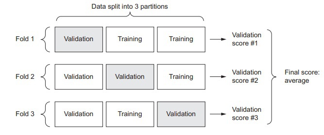
The method of validation we will be using in this example is the K-Fold validation. First things first, we will set aside a portion of samples as our validation dataset. While we are already dealing with a small number of data samples, hence the validation dataset will also be considerably smaller, i.e., a dataset of only 100 samples. In turn, our validation scores will be more prone to changes depending on the data points being used for validation and training. Hence we will be using the K-Fold validation to cover this discrepancy. In K-Fold validation, we basically split the data, which is currently available into partitions known as K-Partitions (K = 4 or 5). After partitioning, we make identical K-models and train the Neural Network on parameters such as K-1 partitions and the evaluations are done on the rest of the partitions, to understand this better, take a look at the demonstration below:
We have coded a K-Fold validation below:
import numpy as np
k=4
num_val_samples = len(train_data) // k
num_epochs = 100
all_scores = []
for i in range(k):
print('processing fold #', i)
val_data = train_data[i * num_val_samples: (i + 1) * num_val_samples]
val_targets = train_targets[i * num_val_samples: (i + 1) * num_val_samples]
partial_train_data = np.concatenate(
[train_data[:i * num_val_samples],
train_data[(i + 1) * num_val_samples:]],
axis=0)
partial_train_targets = np.concatenate(
[train_targets[:i * num_val_samples],
train_targets[(i + 1) * num_val_samples:]],
axis=0)
model = build_model()
model.fit(partial_train_data, partial_train_targets,
epochs=num_epochs, batch_size=1, verbose=0)
val_mse, val_mae = model.evaluate(val_data, val_targets, verbose=0)
all_scores.append(val_mae)
We will specify the number of epochs as 100 by the argument num_epochs = 100
. The corresponding results are shown below:
>>> all_scores
[2.588258957792037, 3.1289568449719116, 3.1856116051248984, 3.0763342615401386]
>>> np.mean(all_scores)
2.9947904173572462
Different number of epochs are giving different results, in our case, ranging from 2.6 to 3.2. The entire purpose of the K-Fold validation is to give a mean of these different scores, which is 3.0 in our case. However, we are still deviating by an average of $3,000 and this is very significant.
We will now try training the network longer, this time for 500 epochs. In addition, we will modify the training session loops such that the performance of the model one each epoch is recorded in a validation score log.
The code to save the validation logs a each fold is as shown below:
num_epochs = 500
all_mae_histories = []
for i in range(k):
print('processing fold #', i)
val_data = train_data[i * num_val_samples: (i + 1) * num_val_samples]
val_targets = train_targets[i * num_val_samples: (i + 1) * num_val_samples]
partial_train_data = np.concatenate(
[train_data[:i * num_val_samples],
train_data[(i + 1) * num_val_samples:]],
axis=0)
partial_train_targets = np.concatenate(
[train_targets[:i * num_val_samples],
train_targets[(i + 1) * num_val_samples:]],
axis=0)
model = build_model()
history = model.fit(partial_train_data, partial_train_targets,
validation_data=(val_data, val_targets),
epochs=num_epochs, batch_size=1, verbose=0)
mae_history = history.history['val_mean_absolute_error']
all_mae_histories.append(mae_history)
To compute and find out the average MAE scores of all the K-Folds, we will use the following lines of code:
average_mae_history = [
np.mean([x[i] for x in all_mae_histories]) for i in range(num_epochs)]
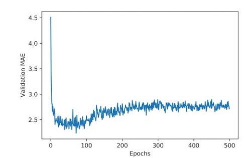
We will now plot the validation scores we have obtained from the Neural network’s training so far and plot it into a graph to analyze the results with more clarity:
import matplotlib.pyplot as plt
plt.plot(range(1, len(average_mae_history) + 1), average_mae_history)
plt.xlabel('Epochs')
plt.ylabel('Validation MAE')
plt.show()
The graphical representation is still unclear because of the issues relating to scaling and frequent variance. To remedy this, we will do the following:
- We will take the initial data points and omit the first 10 that are already on a different scale as compared to the rest of the curve
- We will replace each point in the curve with an exponential moving average. This average is taken from the previous points and will give us a smooth curve.
Now, we will use the following lines of code to plot the validation scores by omitting the initial 10 data points:
def smooth_curve(points, factor=0.9):
smoothed_points = []
for point in points:
if smoothed_points:
previous = smoothed_points[-1]
smoothed_points.append(previous * factor + point * (1 - factor))
else:
smoothed_points.append(point)
return smoothed_points
smooth_mae_history = smooth_curve(average_mae_history[10:])
plt.plot(range(1, len(smooth_mae_history) + 1), smooth_mae_history)
plt.xlabel('Epochs')
plt.ylabel('Validation MAE')
plt.show()
In this graphical representation, we can see that after 80 epochs, the improvement of the validation MAE comes to a halt, and past that, the network experiences overfitting.
Once we have tuned the network on our desired parameters, we can begin testing it with these optimal parameters and check the performance on the testing dataset.
model = build_model()
model.fit(train_data, train_targets,
epochs=80, batch_size=16, verbose=0)
test_mse_score, test_mae_score = model.evaluate(test_data, test_targets)
The final result obtained is:
>>> test_mae_score
2.5532484335057877
We can see that even after all this, the Neural network’s predictions are still off by a value of $2,550.