Chapter 4: Using Deep Learning for Computer Vision
In this chapter, our discussion will revolve around the understanding and visualization of convnets, which are known as convolutional neural networks. The importance of convnets can be estimated from the fact that its use stretches out universally to every computer vision application. After understanding the conceptual realms surrounding convnets, we will proceed to use them practically in problems relating to image-classification. The dataset we will be using in these practical demonstrations will be small, and almost anyone can practice light on computational resources. As such, an example, without needing to arrange resources that are typically available in a big tech company.
What is Convnet? Working with Convolution Operations
Before we begin discussing the details of a convnet, we will first look at a practical demonstration of a deep learning model using a convnet. We will solve the problem of classifying digits in the MNIST dataset (the same task which we demonstrated previously in the second chapter and received an accuracy of 97.8% by using a densely connected Neural network). Compared to the previous method we used for performing this task, implementing a convnet is relatively simple. We will also see how the results of a convnet hold up to a densely connected Neural network.
The following lines of code show how we can instantiate a small convnet in our deep learning model:
from keras import layers
from keras import models
model = models.Sequential()
model.add(layers.Conv2D(32, (3, 3), activation='relu', input_shape=(28, 28, 1)))
model.add(layers.MaxPooling2D((2, 2)))
model.add(layers.Conv2D(64, (3, 3), activation='relu'))
model.add(layers.MaxPooling2D((2, 2)))
model.add(layers.Conv2D(64, (3, 3), activation='relu'))
From the above lines of code, we can see that a typical small convnet is just a stack of two types of layers, namely the Conv2D and MaxPooling2D layers. Regarding the input data, a convnet only accepts tensors that are of the following shape: (image_height, image_width, image_channels). Now we know the shape of the input tensors required, we will configure the convnet accordingly to make it process tensor inputs corresponding to the format of the MNIST images dataset, of the size (28, 28, 1). This can be easily done by using an argument on the first layer. This argument is input_shape (28, 28, 1).
The Network’s architecture will look like this according to the changes we just mentioned:
>>> model.summary()
________________________________________________________________
Layer (type) Output Shape Param #
================================================================
conv2d_1 (Conv2D) (None, 26, 26, 32) 320
________________________________________________________________
maxpooling2d_1 (MaxPooling2D) (None, 13, 13, 32) 0
________________________________________________________________
conv2d_2 (Conv2D) (None, 11, 11, 64) 18496
________________________________________________________________
maxpooling2d_2 (MaxPooling2D) (None, 5, 5, 64) 0
________________________________________________________________
conv2d_3 (Conv2D) (None, 3, 3, 64) 36928
================================================================
Total params: 55,744
Trainable params: 55,744
Non-trainable params: 0
From the network’s architectrure displayed above, we can see that the Conv2D and MaxPooling2D layers output a 3D tensor and the shape of this tensor is (height, width, channels). One more thing to point out is that as we move deeper into the Neural network, the dimensions of width and height will consequently shrink, in addition, the very first argument which we passed on to the layer Conv2D is responsible for controlling the amount of channels in the network.
The next plan of action is to take the output tensor of the last layer and feed it into a classifier network. This classifier network is made up of a stack of dense layers and what they essentially do is take the 1D vectors and process them even though the network is outputting 3D tensors. So, we will proceed to convert the 3D tensors into a 1D tensor and after doing this, we will also throw in a bunch of dense layers, as shown below:
model.add(layers.Flatten())
model.add(layers.Dense(64, activation='relu'))
model.add(layers.Dense(10, activation='softmax'))
In the above lines of code, we are performing a 10-way classification with a softmax activation. Moreover, the classification is being done with the last layer giving 10 outputs. The Neural network thus far looks like this:
>>> model.summary()
Layer (type) Output Shape Param #
================================================================
conv2d_1 (Conv2D) (None, 26, 26, 32) 320
________________________________________________________________
maxpooling2d_1 (MaxPooling2D) (None, 13, 13, 32) 0
________________________________________________________________
conv2d_2 (Conv2D) (None, 11, 11, 64) 18496
________________________________________________________________
maxpooling2d_2 (MaxPooling2D) (None, 5, 5, 64) 0
________________________________________________________________
conv2d_3 (Conv2D) (None, 3, 3, 64) 36928
________________________________________________________________
flatten_1 (Flatten) (None, 576) 0
________________________________________________________________
dense_1 (Dense) (None, 64) 36928
________________________________________________________________
dense_2 (Dense) (None, 10) 650
================================================================
Total params: 93,322
Trainable params: 93,322
Non-trainable params: 0
We will now start training of the convnet Neural network on the MNIST training set. You will notice most of the code being repeated from the example in chapter 2.
from keras.datasets import mnist
from keras.utils import to_categorical
(train_images, train_labels), (test_images, test_labels) = mnist.load_data()
train_images = train_images.reshape((60000, 28, 28, 1))
train_images = train_images.astype('float32') / 255
test_images = test_images.reshape((10000, 28, 28, 1))
test_images = test_images.astype('float32') / 255
train_labels = to_categorical(train_labels)
test_labels = to_categorical(test_labels)
model.compile(optimizer='rmsprop',
loss='categorical_crossentropy',
metrics=['accuracy'])
model.fit(train_images, train_labels, epochs=5, batch_size=64)
Now to evaluate the deep learning model after training it:
>>> test_loss, test_acc = model.evaluate(test_images, test_labels)
>>> test_acc
0.99080000000000001
So from the above results, we can see that by using a convnet on the same MNIST dataset, we get an accuracy of 99.3% as compared to the 97.8% accuracy by using a densely connected network.
The reason for this improvement in accuracy is because of the Conv2D and MaxPooling2D layers, and to understand this better, we will discuss these two layers in detail.
The Convolution Operation (CONV2D)
Let’s talk about what makes a convolution layer different from a densely connected layer. The most fundamental difference between these two comes in their learning patterns. While a dense layer takes the approach of learning a global pattern within the input space, on the other hand, a convolution layer does the opposite, i.e., it learns a local pattern.
Due to this characteristic of convnets, they have developed the following two important properties:
- The patterns learned by convnets are translation invariant. This means that when a convnet is finished with learning a particular pattern, let’s say, in the upper-left corner of a drawing or a picture, it can then detect and recognize this particular pattern in any location of the picture. This is where a densely connected network falls behind as for it to recognize the same pattern in a new location, it will have to learn it from scratch. Hence, in terms of image processing, convnets are not only data efficient, but they are also resource-efficient as well as they only require a small number of training samples to learn those representations that have a much-needed generalization power.
- Convnets can learn the spatial hierarchies of patterns. The visual world is in nature, spatially hierarchical, hence making this property of convnets very important. The learning process works as follows: in a convnet, there are several convolution layers. Based on the hierarchical position of these layers, they learn different patterns.
The first convolutional layer will only learn small local patterns, while the second convolutional layer will learn bigger local patterns that have the same features as the smaller ones. In this way, a convnet is capable of not only learning increasingly complex patterns, but it can also learn abstract concepts.
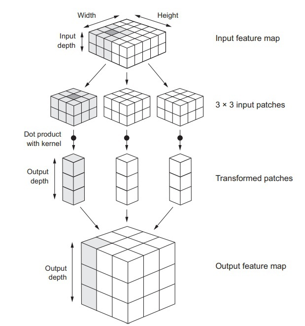
Convolutional operations work on 3D tensors. This tensor is known as a “feature map.” This tensor has two spatial axes and a depth axis. In other words, a convolution operation takes out a patch from this inputted feature map and applies this transformation on all of the other patches. In this way, the network obtains an output feature map from an input feature map.
Furthermore, the following two parameters define convolutions:
- Size of the patches taken from the input feature map. This size is either 3x3 or 5x5.
- The output feature map’s depth refers to the number of filters that have been computed by the convolution operation.
You can see these parameters in Keras as well so much so that they are the very first arguments which are passed to the convolution layers as:
Conv2D(output_depth, (window_height, window_width))
The size of the windows, as shown in the argument above, can be either 3x3 or 5x5. What the convolution operation does in this argument is that it “slides” the windows mentioned above over a given 3D input feature map. During the sliding, the operation searches for 3D patches that have the corresponding features (shape (window_height, window_width, input_depth)), and wherever it finds such a 3D patch, it stops and extracts this 3D patch. Once a 3D patch has been extracted, it is converted into a 1D vector with shape (output_depth). Once enough 3D patches have been extracted and converted into 1D vectors, the next plan of action is for the convolution is to reassemble them into a 3D feature map spatially. This is the output feature map. The shape of this 3D feature map would be (height, width, output_depth). To understand this concept better, take a look at the visualization of how convolutions work.
(The Working of a Convolution)
Some characteristics of the output feature map may be different from the input feature map, such as the height and width, this is because of two main reasons:
- Border effects (This can be remedied by padding the input feature map).
- Using strides.
The MaxPooling2D Operation
The main job of the MaxPooling2D operation is to downsample the feature maps. In the previous examples of convolution operations, we can see that initially, the size of the feature map was 26x26, but as soon as it passed through the maxpooling2D layer, the size of the feature map was downsampled to 13x13.
Conceptually, the max-pooling operation is similar to the convolution operation, the point where this similarity comes to an end is when both of the operations need to convert the local patches. A convolution operation does this by using a convolution kernel (basically an already learned linear transformation) while, on the other hand, a max-pooling operation performs this transformation by using a max
tensor operation, which is hardcoded. One more big difference between the two operations is that max-pooling is most of the time, done with windows of the size 2x2 and stride 2 while a convolution is done with a window that has a size of 3x3. Moreover, no stride is used (stride 1).
You might be wondering that what is the point of even downsampling the feature maps in the first place. To answer this, let’s look at a convolutional base model without a downsized feature map:
model_no_max_pool = models.Sequential()
model_no_max_pool.add(layers.Conv2D(32, (3, 3), activation='relu',
input_shape=(28, 28, 1)))
model_no_max_pool.add(layers.Conv2D(64, (3, 3), activation='relu'))
model_no_max_pool.add(layers.Conv2D(64, (3, 3), activation='relu'))
The summary of this model is as follows:
>>> model_no_max_pool.summary()
Layer (type) Output Shape Param #
================================================================
conv2d_4 (Conv2D) (None, 26, 26, 32) 320
________________________________________________________________
conv2d_5 (Conv2D) (None, 24, 24, 64) 18496
________________________________________________________________
conv2d_6 (Conv2D) (None, 22, 22, 64) 36928
================================================================
Total params: 55,744
Trainable params: 55,744
Non-trainable params: 0
After analyzing this model, we come to know that two major things are wrong with this particular setup:
- This setup is not optimal in regards to learning a feature’s spatial hierarchy. This is because the window in the network’s third layer is of the size 3x3, and it will only contain information that is coming from the initial input, and the size of this window is 7x7. Hence, we require the features of the convolution layer to store the information pertaining to the input’s totality.
- The setup is unnecessarily large for our purposes of a small deep learning model. This setup’s final feature map has an enormous number of coefficients, i.e., 22 x 22 x 64 which per sample, equals to a total of 30,976 coefficients. Now, if we want to add a dense layer on this model, then we would first need to flatten the feature map. So let’s say we do flatten it out and put a size 512 dense layer on top of it, the resulting parameters of the layer would be around 15.8 million. This would result in overfitting of the model.
So, the essence of downsampling is just to cut down the number of coefficients our feature map has, besides, downsampling also creates a kind of filter for spatial hierarchies. This is done by arranging successive convolutional layers in such a way that they progressively deal with larger windows.
Training a Convnet
In computer vision, the most common task for which deep learning models are used for is image-classification. Hence, we will be training our deep learning model using a convnet on a dataset consisting of 4,000 picture samples of cats and dogs. The task which is to be performed by the network is to learn to recognize dogs and cats separately in the picture samples. As always, we divide the 4,000 samples between training, validation, and testing. 2,000 samples will be used for training the network, 1,000 samples will be used as the validation set, and the remaining 1,000 samples will be used as the testing set.
As we are working with a considerably small dataset, we will need to strategize the training of the network accordingly. At first, we will not consider any regularization while training the convnet with the 2,000 sample training dataset. By doing so, we will essentially establish a baseline detailing the limits of what is the network is capable of. The classification accuracy thus obtained will be a measly 71%, with the main point of concern being overfitting. We will then proceed to diminish this overfitting as much as possible by using a rather robust and potent technique known as “data augmentation.” This will bring the classification accuracy of the convnet up to 81%, a sizeable difference as compared to before.
This is all which will be covered in this section. In the following sections of this chapter, we will discuss another pair of techniques that help us implement deep learning models on small datasets which are:
- Feature extraction with a pertained network. (Accuracy of 90-96%)
- Fine-tuning a pertained network. (Accuracy of 97%).
By combining these two techniques with the one we have just discussed, you can develop a very powerful toolbox for handling image-classification problems anytime and anywhere.
Downloading the Data
The very first thing to do is to obtain the data on which we will train and build our deep learning model’s network. We will be using a dataset released by Kaggle, and this dataset is known as the Dogs vs. Cats dataset. This dataset does not come packaged in Keras. Hence we will need to download it from Kaggle’s website. Also, before you can download the dataset, you will need to create a Kaggle account if you don’t have one.
www.kaggle.com/c/dogs-vs-cats/data
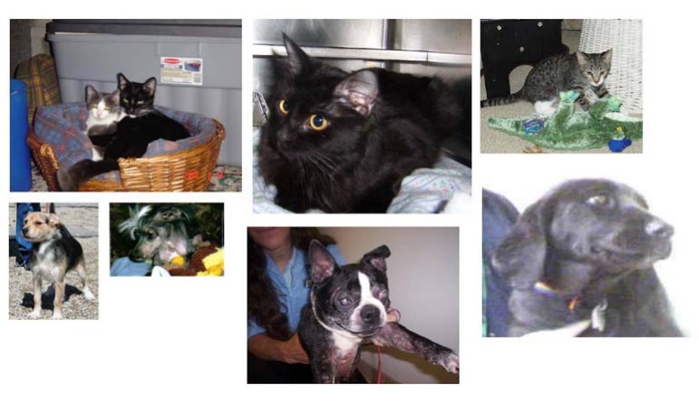
The pictures included in this dataset are in a JPEG format, and they are of medium resolution. Some examples of the pictures included in this dataset are shown below (the pictures shown are not modified or edited, they differ in sizes to make the dataset heterogenous):
Although the dataset consists of a total of 25,000 pictures (12,500 dogs and 12,500 cats), we will be only using a total of 4,000 samples in accordance to the training, validation and testing sets we discussed beforehand. If we work with a large dataset, then it would defeat the purpose of using deep learning for small datasets.
Hence, we will divide the dataset accordingly: 1,000 samples of each class (dogs and cats) for our training dataset, 500 samples of each class for our validation dataset, and 500 samples of each class for the testing dataset.
To copy these samples to their corresponding training, validation and testing directories, we will use the following lines of code:
import os, shutil
original_dataset_dir = '/Users/fchollet/Downloads/kaggle_original_data'
base_dir = '/Users/fchollet/Downloads/cats_and_dogs_small'
os.mkdir(base_dir)
train_dir = os.path.join(base_dir, 'train')
os.mkdir(train_dir)
validation_dir = os.path.join(base_dir, 'validation')
os.mkdir(validation_dir)
test_dir = os.path.join(base_dir, 'test')
os.mkdir(test_dir)
train_cats_dir = os.path.join(train_dir, 'cats')
os.mkdir(train_cats_dir)
train_dogs_dir = os.path.join(train_dir, 'dogs')
os.mkdir(train_dogs_dir)
validation_cats_dir = os.path.join(validation_dir, 'cats')
os.mkdir(validation_cats_dir)
validation_dogs_dir = os.path.join(validation_dir, 'dogs')
os.mkdir(validation_dogs_dir)
test_cats_dir = os.path.join(test_dir, 'cats')
os.mkdir(test_cats_dir)
test_dogs_dir = os.path.join(test_dir, 'dogs')
os.mkdir(test_dogs_dir)
fnames = ['cat.{}.jpg'.format(i) for i in range(1000)]
for fname in fnames:
src = os.path.join(original_dataset_dir, fname)
dst = os.path.join(train_cats_dir, fname)
shutil.copyfile(src, dst)
fnames = ['cat.{}.jpg'.format(i) for i in range(1000, 1500)]
for fname in fnames:
src = os.path.join(original_dataset_dir, fname)
dst = os.path.join(validation_cats_dir, fname)
shutil.copyfile(src, dst)
fnames = ['cat.{}.jpg'.format(i) for i in range(1500, 2000)]
for fname in fnames:
src = os.path.join(original_dataset_dir, fname)
dst = os.path.join(test_cats_dir, fname)
shutil.copyfile(src, dst)
fnames = ['dog.{}.jpg'.format(i) for i in range(1000)]
for fname in fnames:
src = os.path.join(original_dataset_dir, fname)
dst = os.path.join(train_dogs_dir, fname)
shutil.copyfile(src, dst)
fnames = ['dog.{}.jpg'.format(i) for i in range(1000, 1500)]
for fname in fnames:
src = os.path.join(original_dataset_dir, fname)
dst = os.path.join(validation_dogs_dir, fname)
shutil.copyfile(src, dst)
fnames = ['dog.{}.jpg'.format(i) for i in range(1500, 2000)]
for fname in fnames:
src = os.path.join(original_dataset_dir, fname)
dst = os.path.join(test_dogs_dir, fname)
shutil.copyfile(src, dst)
We will now double check number of pictures in each directory:
>>> print('total training cat images:', len(os.listdir(train_cats_dir)))
total training cat images: 1000
>>> print('total training dog images:', len(os.listdir(train_dogs_dir)))
total training dog images: 1000
>>> print('total validation cat images:', len(os.listdir(validation_cats_dir)))
total validation cat images: 500
>>> print('total validation dog images:', len(os.listdir(validation_dogs_dir)))
total validation dog images: 500
>>> print('total test cat images:', len(os.listdir(test_cats_dir)))
total test cat images: 500
>>> print('total test dog images:', len(os.listdir(test_dogs_dir)))
total test dog images: 500
So far, everything looks good and in place. We will now proceed to build the network as we have obtained the necessary data.
Building the Network
As we have already built a small yet simple convnet for an MNIST dataset, we will be using the same general structure, i.e., the stack of layers being used will be an alternating arrangement of Conv2D
and MaxPooling2D
layers. The convolution operation will be using a relu activation function. However, we will be adding another Conv2D and MaxPooling2D layer to make the network larger because, unlike before, we are now dealing with a more complex problem and larger images. By doing so, we will not only be augmenting the capacity of the network we are building, but we will also be able to reduce the size of the feature maps even further before we reach the point of the flatten
layer. Following this concept, we will be starting from inputs with a size of 150x150 and ending up feature maps of the size 7x7 right before the flatten
layer.
By using common sense, we can see that the nature of the problem we are tackling is, in essence, a binary classification problem. Just as how we dealt with such problems in the previous chapters, we will be using a size 1 dense layer with a sigmoid activation function to end our network, hence encoding the probability of whether the network is looking at a picture of a dog or a cat.
The network will be built as follows:
from keras import layers
from keras import models
model = models.Sequential()
model.add(layers.Conv2D(32, (3, 3), activation='relu',
input_shape=(150, 150, 3)))
model.add(layers.MaxPooling2D((2, 2)))
model.add(layers.Conv2D(64, (3, 3), activation='relu'))
model.add(layers.MaxPooling2D((2, 2)))
model.add(layers.Conv2D(128, (3, 3), activation='relu'))
model.add(layers.MaxPooling2D((2, 2)))
model.add(layers.Conv2D(128, (3, 3), activation='relu'))
model.add(layers.MaxPooling2D((2, 2)))
model.add(layers.Flatten())
model.add(layers.Dense(512, activation='relu'))
model.add(layers.Dense(1, activation='sigmoid'))
While we are at it, let’s take a sneak peek at how the dimensions of the feature maps are changing through every succeeding layer they go through:
>>> model.summary()
Layer (type) Output Shape Param #
================================================================
conv2d_1 (Conv2D) (None, 148, 148, 32) 896
________________________________________________________________
maxpooling2d_1 (MaxPooling2D) (None, 74, 74, 32) 0
________________________________________________________________
conv2d_2 (Conv2D) (None, 72, 72, 64) 18496
________________________________________________________________
maxpooling2d_2 (MaxPooling2D) (None, 36, 36, 64) 0
________________________________________________________________
conv2d_3 (Conv2D) (None, 34, 34, 128) 73856
________________________________________________________________
maxpooling2d_3 (MaxPooling2D) (None, 17, 17, 128) 0
________________________________________________________________
conv2d_4 (Conv2D) (None, 15, 15, 128) 147584
________________________________________________________________
maxpooling2d_4 (MaxPooling2D) (None, 7, 7, 128) 0
________________________________________________________________
flatten_1 (Flatten) (None, 6272) 0
________________________________________________________________
dense_1 (Dense) (None, 512) 3211776
________________________________________________________________
dense_2 (Dense) (None, 1) 513
================================================================
Total params: 3,453,121
Trainable params: 3,453,121
Non-trainable params: 0
We are using a network that ends with a singular sigmoid unit, hence the loss function which we will be using for the network is crossentropy. The optimizer used will be rmsprop.
We will configure the network accordingly:
from keras import optimizers
model.compile(loss='binary_crossentropy',
optimizer=optimizers.RMSprop(lr=1e-4),
metrics=['acc'])
Preprocessing the Data
As is the case with building Neural networks, we will now proceed to convert the data into the appropriate preprocessed floating-point tensors. This will be done as follows:
- Go through the pictures in the sample data
- Decode these pictures which are in a JPEG format into pixels on RGB grids
- Convert these pixels into floating-point tensors
- Rescale the values of the resulting pixels into the (0, 1) interval
Fortunately, we will not have to perform these steps entirely manually. Keras has the necessary utilities to help us perform these steps as shown in the code below:
from keras.preprocessing.image import ImageDataGenerator
train_datagen = ImageDataGenerator(rescale=1./255)
test_datagen = ImageDataGenerator(rescale=1./255)
train_generator = train_datagen.flow_from_directory(
train_dir,
target_size=(150, 150)
batch_size=20,
class_mode='binary')
validation_generator = test_datagen.flow_from_directory(
validation_dir,
target_size=(150, 150),
batch_size=20,
class_mode='binary')
The image data generator used in this code will keep generating these data batches infinitely. Now we will break the generating loop once we have gotten the converted data:
>>> for data_batch, labels_batch in train_generator:
>>> print('data batch shape:', data_batch.shape)
>>> print('labels batch shape:', labels_batch.shape)
>>> break
data batch shape: (20, 150, 150, 3)
labels batch shape: (20,)
Now, to fit the deep learning model using a batch generator:
history = model.fit_generator(
train_generator,
steps_per_epoch=100,
epochs=30,
validation_data=validation_generator,
validation_steps=50)
Never a bad idea to save the model:
model.save('cats_and_dogs_small_1.h5')
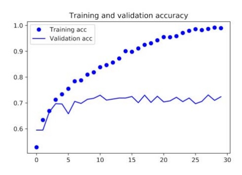
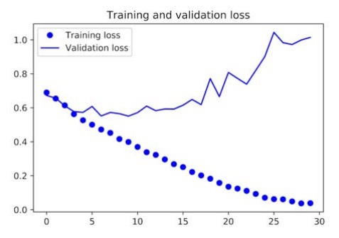
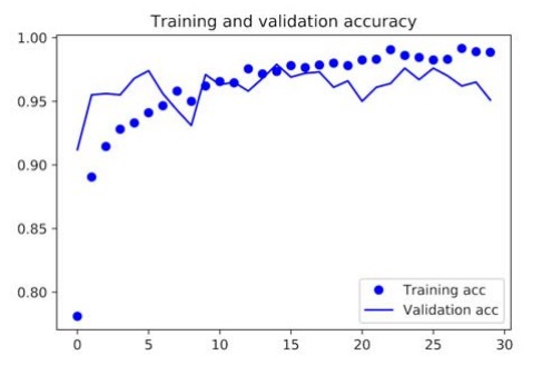
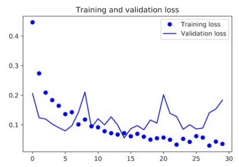
We will now plot the loss and accuracy data of this deep learning model to analyze it and make changes to the model accordingly:
import matplotlib.pyplot as plt
acc = history.history['acc']
val_acc = history.history['val_acc']
loss = history.history['loss']
val_loss = history.history['val_loss']
epochs = range(1, len(acc) + 1)
plt.plot(epochs, acc, 'bo', label='Training acc')
plt.plot(epochs, val_acc, 'b', label='Validation acc')
plt.title('Training and validation accuracy')
plt.legend()
plt.figure()
plt.plot(epochs, loss, 'bo', label='Training loss')
plt.plot(epochs, val_loss, 'b', label='Validation loss')
plt.title('Training and validation loss')
plt.legend()
plt.show()
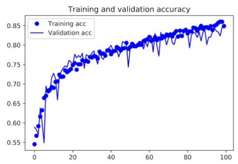
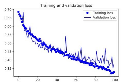
By running this code, we get the following graphical representations of the loss and accuracy data of the model:
In our current model, the problem of overfitting is the main concern at this point. We have learned several techniques to deal with overfittings, such as the weight decay method and the dropout method. However, in this example, we will be using a new technique known as data augmentation, and this technique is used almost universally for deep learning models that are dealing with image-classification tasks.
Mitigating Overfitting by Data Augmentation
Overfitting is very prominent in models that are using a small number of samples for training their Neural network. Data augmentation diminishes overfitting by opting for the approach that, if we have a larger number of training samples, then there will be less overfitting. Hence data augmentation generates new training samples from the existing set of training samples through randomly transforming data into similarly structured data (known as augmentation).
We will now establish a data augmentation configuration for our model using the ImageDataGenerator function:
datagen = ImageDataGenerator(
rotation_range=40,
width_shift_range=0.2,
height_shift_range=0.2,
shear_range=0.2,
zoom_range=0.2,
horizontal_flip=True,
fill_mode='nearest')
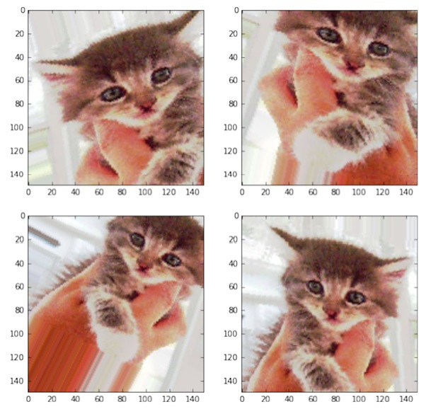
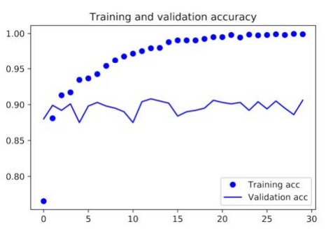
Now to display some of the augmented images which we have created for the network’s training:
from keras.preprocessing import image
fnames = [os.path.join(train_cats_dir, fname) for
fname in os.listdir(train_cats_dir)]
img_path = fnames[3]
img = image.load_img(img_path, target_size=(150, 150))
x = image.img_to_array(img)
x = x.reshape((1,) + x.shape)
i=0
for batch in datagen.flow(x, batch_size=1):
plt.figure(i)
imgplot = plt.imshow(image.array_to_img(batch[0]))
i += 1
if i % 4 == 0:
break
plt.show()
These are the cat pictures that have been generated through data augmentation. However, this will not completely diminish overfitting because we are just remixing the existing information and training the network on it, so no new data is being produced. To further reduce overfitting in the model, we will add in a dropout
layer and place it just before the densely connected classifier.
We will now define a convnet and this time, it will include the dropout layer:
model = models.Sequential()
model.add(layers.Conv2D(32, (3, 3), activation='relu',
input_shape=(150, 150, 3)))
model.add(layers.MaxPooling2D((2, 2)))
model.add(layers.Conv2D(64, (3, 3), activation='relu'))
model.add(layers.MaxPooling2D((2, 2)))
model.add(layers.Conv2D(128, (3, 3), activation='relu'))
model.add(layers.MaxPooling2D((2, 2)))
model.add(layers.Conv2D(128, (3, 3), activation='relu'))
model.add(layers.MaxPooling2D((2, 2)))
model.add(layers.Flatten())
model.add(layers.Dropout(0.5))
model.add(layers.Dense(512, activation='relu'))
model.add(layers.Dense(1, activation='sigmoid'))
model.compile(loss='binary_crossentropy',
optimizer=optimizers.RMSprop(lr=1e-4),
metrics=['acc'])
Now to train the network by using data augmentation and dropout:
train_datagen = ImageDataGenerator(
rescale=1./255,
rotation_range=40,
width_shift_range=0.2,
height_shift_range=0.2,
shear_range=0.2,
zoom_range=0.2,
horizontal_flip=True,)
test_datagen = ImageDataGenerator(rescale=1./255)
train_generator = train_datagen.flow_from_directory(
train_dir,
target_size=(150, 150),
batch_size=32,
class_mode='binary')
validation_generator = test_datagen.flow_from_directory(
validation_dir,
target_size=(150, 150),
batch_size=32,
class_mode='binary')
history = model.fit_generator(
train_generator,
steps_per_epoch=100,
epochs=100,
validation_data=validation_generator,
validation_steps=50)
A very important note, never augment the validation data.
Let’s save the model in case we need it for future purposes:
model.save('cats_and_dogs_small_2.h5')
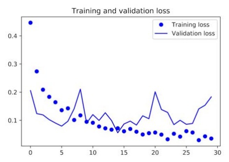
The following are the results plotted onto a graph:
We can see that the training curves are closely following the validation curves, and we have eradicated overfitting from our deep learning model by using data augmentation and dropout.
Working with a Pretrained Convnet
This another effective, efficient, and very commonly practiced approach for people using deep learning models in computer vision. This approach is self-definitive. We are using a convnet that has already been trained on a large-scale dataset used primarily for tackling a complex and huge image-classification task, and later, this network has been saved. We can use this network for small datasets with a little change here and there. Moreover, a pre-trained convnet most probably has a sizable spatial hierarchy learned, meaning that it can perform general classification.
A pre-trained network can be used by following either of the two ways;
- Feature Extraction
- Fine Tuning
Feature Extraction
In feature extraction, we use representations of the pre-trained convnet to extract some new features in the current dataset we are working on. Once the features have been extracted, we then train a new classifier and run these features through it.
To refresh our memory, a typical convnet begins with a bunch of convolution and max-pooling layers and end with a densely connected classifier. In feature extraction, we will use the convolutional base of the pre-trained convnet and run our data through it. Afterward, we will train a new classifier and put it on top of the output yielded by the pre-trained convnets convolutional base.
We are essentially swapping out the pre-trained convnet's classifier with a newly trained classifier while keeping the same convolutional base as shown below;
Let’s being using a pre-trained convnet. There are several pre-trained convnets models available in Keras which are;
- Xception
- Inception V3
- ResNet50
- VGG16
- VGG19
- MobileNet
We will be using a VGG16 convnet, which has been pre-trained on the ImageNet dataset. As per feature extraction, we will be extracting the features of cats and dogs from this convnet’s convolutional base. After extracting the features, we will train a dog vs. cat classifier and place it on these extracted features.
We do not need to download the VGG16 model as it is already available for use in Keras. To import it, we will use the module keras.applications
.
We will now proceed to begin instantiating the convolutional base of VGG16;
from keras.applications import VGG16
conv_base = VGG16(weights='imagenet',
include_top=False,
input_shape=(150, 150, 3))
To understand the VGG16’s convolutional base better, take a look at a detailed architecture of it;
>>> conv_base.summary()
Layer (type) Output Shape Param #
================================================================
input_1 (InputLayer) (None, 150, 150, 3) 0
________________________________________________________________
block1_conv1 (Convolution2D) (None, 150, 150, 64) 1792
________________________________________________________________
block1_conv2 (Convolution2D) (None, 150, 150, 64) 36928
________________________________________________________________
block1_pool (MaxPooling2D) (None, 75, 75, 64) 0
________________________________________________________________
block2_conv1 (Convolution2D) (None, 75, 75, 128) 73856
________________________________________________________________
block2_conv2 (Convolution2D) (None, 75, 75, 128) 147584
________________________________________________________________
block2_pool (MaxPooling2D) (None, 37, 37, 128) 0
________________________________________________________________
block3_conv1 (Convolution2D) (None, 37, 37, 256) 295168
________________________________________________________________
block3_conv2 (Convolution2D) (None, 37, 37, 256) 590080
________________________________________________________________
block3_conv3 (Convolution2D) (None, 37, 37, 256) 590080
________________________________________________________________
block3_pool (MaxPooling2D) (None, 18, 18, 256) 0
________________________________________________________________
block4_conv1 (Convolution2D) (None, 18, 18, 512) 1180160
________________________________________________________________
block4_conv2 (Convolution2D) (None, 18, 18, 512) 2359808
________________________________________________________________
block4_conv3 (Convolution2D) (None, 18, 18, 512) 2359808
________________________________________________________________
block4_pool (MaxPooling2D) (None, 9, 9, 512) 0
________________________________________________________________
block5_conv1 (Convolution2D) (None, 9, 9, 512) 2359808
________________________________________________________________
block5_conv2 (Convolution2D) (None, 9, 9, 512) 2359808
________________________________________________________________
block5_conv3 (Convolution2D) (None, 9, 9, 512) 2359808
________________________________________________________________
block5_pool (MaxPooling2D) (None, 4, 4, 512) 0
================================================================
Total params: 14,714,688
Trainable params: 14,714,688
Non-trainable params: 0
As we can see the final block has a feature map of (4, 4, 512). We will place a densely connected classifier on top of this feature map.
Now we can proceed with feature extraction in two ways;
- Feature extraction without data augmentation
- Feature extraction with data augmentation
Feature Extraction Without Data Augmentation
This method is particularly suitable in cases where you do not have access to a GPU, or you can only run your code on the CPU. First of all, we will begin by extracting the images along with their labels as NumPy arrays by using the ImageDataGenerator. The features will be extracted by using the predict
method of the conv_base
model.
import os
import numpy as np
from keras.preprocessing.image import ImageDataGenerator
base_dir = '/Users/fchollet/Downloads/cats_and_dogs_small'
train_dir = os.path.join(base_dir, 'train')
validation_dir = os.path.join(base_dir, 'validation')
test_dir = os.path.join(base_dir, 'test')
datagen = ImageDataGenerator(rescale=1./255)
batch_size = 20
def extract_features(directory, sample_count):
features = np.zeros(shape=(sample_count, 4, 4, 512))
labels = np.zeros(shape=(sample_count))
generator = datagen.flow_from_directory(
directory,
target_size=(150, 150),
batch_size=batch_size,
class_mode='binary')
i=0
for inputs_batch, labels_batch in generator:
features_batch = conv_base.predict(inputs_batch)
features[i * batch_size : (i + 1) * batch_size] = features_batch
labels[i * batch_size : (i + 1) * batch_size] = labels_batch
i += 1
if i * batch_size >= sample_count:
break
return features, labels
train_features, train_labels = extract_features(train_dir, 2000)
validation_features, validation_labels = extract_features(validation_dir, 1000)
test_features, test_labels = extract_features(test_dir, 1000)
Since we are now going to use a densely connected classifier on the extracted features, we will first need to flatten their shape. The shape of the extracted features is (4, 4, 512) and we will flatten this shape into (samples, 8192) as shown below;
train_features = np.reshape(train_features, (2000, 4*4* 512))
validation_features = np.reshape(validation_features, (1000, 4*4* 512))
test_features = np.reshape(test_features, (1000, 4*4* 512))
Now that we have the required form of input for the densely connected classifier, we can now define it and use the training data and labels we recently recorded for training this classifier;
from keras import models
from keras import layers
from keras import optimizers
model = models.Sequential()
model.add(layers.Dense(256, activation='relu', input_dim=4 * 4 * 512))
model.add(layers.Dropout(0.5))
model.add(layers.Dense(1, activation='sigmoid'))
model.compile(optimizer=optimizers.RMSprop(lr=2e-5),
loss='binary_crossentropy',
metrics=['acc'])
history = model.fit(train_features, train_labels,
epochs=30,
batch_size=20,
validation_data=(validation_features, validation_labels))
Since we are only using two dense layers, hence, the speed of the training is very speedy such that the time taken by each epoch to complete is lesser than a second even though we are running our code only on the CPU.
Now, we will analyze the loss and accuracy of the model by plotting it graphically;
import matplotlib.pyplot as plt
acc = history.history['acc']
val_acc = history.history['val_acc']
loss = history.history['loss']
val_loss = history.history['val_loss']
epochs = range(1, len(acc) + 1)
plt.plot(epochs, acc, 'bo', label='Training acc')
plt.plot(epochs, val_acc, 'b', label='Validation acc')
plt.title('Training and validation accuracy')
plt.legend()
plt.figure()
plt.plot(epochs, loss, 'bo', label='Training loss')
plt.plot(epochs, val_loss, 'b', label='Validation loss')
plt.title('Training and validation loss')
plt.legend()
plt.show()
By using a pre-trained convnet, we reached a validation accuracy of 90% on our first go without using data augmentation for eradicating the overfitting.
Feature Extraction with Data Augmentation
Apart from the fact that in this method, we will implement data augmentation into the convnet, this method is recommended to be used only if the machine has access to a GPU as it is very resource-intensive. Generally, feature extraction is a slower and expensive process, but the upside to this method is that we can use data augmentation. Feature extraction without data augmentation is faster, and a little less resource-intensive, so bear this in mind when choosing which method to go for.
We will first add the conv_base model to the sequential models just as how we would add layers on top of each other;
from keras import models
from keras import layers
model = models.Sequential()
model.add(conv_base)
model.add(layers.Flatten())
model.add(layers.Dense(256, activation='relu'))
model.add(layers.Dense(1, activation='sigmoid'))
The architecture summary of the model so far is;
>>> model.summary()
Layer (type) Output Shape Param #
================================================================
vgg16 (Model) (None, 4, 4, 512) 14714688
________________________________________________________________
flatten_1 (Flatten) (None, 8192) 0
________________________________________________________________
dense_1 (Dense) (None, 256) 2097408
________________________________________________________________
dense_2 (Dense) (None, 1) 257
================================================================
Total params: 16,812,353
Trainable params: 16,812,353
Non-trainable params: 0
From the model summary, we can see that the VGG16 model’s convolutional base has over a million parameters and the densely connected classifier we are adding has 2 million parameters. In such a scenario, we can just freeze the convolutional base before proceeding with the training and compilation of the model.
Freezing a network can be done in Keras by simply setting the trainable
attribute of the network to false
as shown below;
>>> print('This is the number of trainable weights '
'before freezing the conv base:', len(model.trainable_weights))
This is the number of trainable weights before freezing the conv base: 30
>>> conv_base.trainable = False
>>> print('This is the number of trainable weights '
'after freezing the conv base:', len(model.trainable_weights))
This is the number of trainable weights after freezing the conv base: 4
To bring the changes we just made into effect, we first need to compile the model; otherwise, the changes will be ignored. After compiling and applying this change to the model, we will now start training the model with a frozen convolutional base;
from keras.preprocessing.image import ImageDataGenerator
from keras import optimizers
train_datagen = ImageDataGenerator(
rescale=1./255,
rotation_range=40,
width_shift_range=0.2,
height_shift_range=0.2,
shear_range=0.2,
zoom_range=0.2,
horizontal_flip=True,
fill_mode='nearest')
test_datagen = ImageDataGenerator(rescale=1./255)
train_generator = train_datagen.flow_from_directory(
train_dir,
target_size=(150, 150),
batch_size=20,
class_mode='binary')
validation_generator = test_datagen.flow_from_directory(
validation_dir,
target_size=(150, 150),
batch_size=20,
class_mode='binary')
model.compile(loss='binary_crossentropy',
optimizer=optimizers.RMSprop(lr=2e-5),
metrics=['acc'])
history = model.fit_generator(
train_generator,
steps_per_epoch=100,
epochs=30,
validation_data=validation_generator,
validation_steps=50)
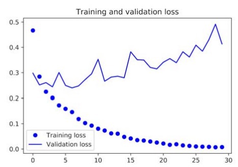
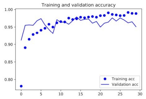
Now let’s see the results after plotting the loss and accuracy of the model;
From the above curves, we can see that the validation accuracy of the model is a whopping 96%. Really big improvement as compared to the convnet we trained on a small dataset.
Fine Tuning
We will try to keep this as brief and to the point as possible because it correlates to the concepts we discussed previously in feature extraction.
A pre-trained convnet can be used by the method of fine-tuning, which is essentially the unfreezing of the top layers which have been frozen when using the feature extraction method. After unfreezing, we train these top layers and the new fully-connected classifier. In essence, we are taking the pre-trained convnet and adjusting its abstract representations ever so slightly to increase the relevance of the representations for the current task.
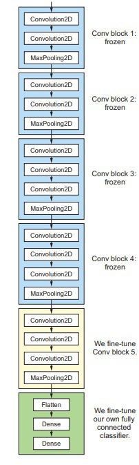
Here’s a visual representation of how a last convolutional block of the VGG16 convnet is fine-tuned;
An important note to remember in fine-tuning is that it is necessary to train the classifier before adding it to the top layers. Otherwise, during training, there will be a huge error signal propagating through the entire network, eradicating the representations which have been previously learned by the layers that we are fine-tuning. Hence, it is important to follow these steps to fine-tune a pre-trained convnet properly;
- When taking a pre-trained network, put in your custom network on top of it.
- Then proceed to freeze the first network (the base).
- Proceed with training the custom network which you recently added.
- Go to the frozen base network and unfreeze some of the layers in there.
- Finally, train these unfrozen layers and the recently added custom network together.
In feature extraction, we performed the initial 3 steps, in fine-tuning we will have to perform all of these steps. As we already know how to perform the first 3 steps, let’s start directly on step 4 i.e, unfreezing the conv_base and freezing some of the individual layers of this model. The summary of our model so far should look like this;
>>> conv_base.summary()
Layer (type) Output Shape Param #
================================================================
input_1 (InputLayer) (None, 150, 150, 3) 0
________________________________________________________________
block1_conv1 (Convolution2D) (None, 150, 150, 64) 1792
________________________________________________________________
block1_conv2 (Convolution2D) (None, 150, 150, 64) 36928
________________________________________________________________
block1_pool (MaxPooling2D) (None, 75, 75, 64) 0
________________________________________________________________
block2_conv1 (Convolution2D) (None, 75, 75, 128) 73856
________________________________________________________________
block2_conv2 (Convolution2D) (None, 75, 75, 128) 147584
________________________________________________________________
block2_pool (MaxPooling2D) (None, 37, 37, 128) 0
________________________________________________________________
block3_conv1 (Convolution2D) (None, 37, 37, 256) 295168
________________________________________________________________
block3_conv2 (Convolution2D) (None, 37, 37, 256) 590080
________________________________________________________________
block3_conv3 (Convolution2D) (None, 37, 37, 256) 590080
________________________________________________________________
block3_pool (MaxPooling2D) (None, 18, 18, 256) 0
________________________________________________________________
block4_conv1 (Convolution2D) (None, 18, 18, 512) 1180160
________________________________________________________________
block4_conv2 (Convolution2D) (None, 18, 18, 512) 2359808
________________________________________________________________
block4_conv3 (Convolution2D) (None, 18, 18, 512) 2359808
________________________________________________________________
block4_pool (MaxPooling2D) (None, 9, 9, 512) 0
________________________________________________________________
block5_conv1 (Convolution2D) (None, 9, 9, 512) 2359808
________________________________________________________________
block5_conv2 (Convolution2D) (None, 9, 9, 512) 2359808
________________________________________________________________
block5_conv3 (Convolution2D) (None, 9, 9, 512) 2359808
________________________________________________________________
block5_pool (MaxPooling2D) (None, 4, 4, 512) 0
================================================================
Total params: 14714688
From this model, we will be fine-tuning only the ending three layers and freeze the rest of the layers up till block4_pool will be frozen.
We will now freeze all of the layers until the block5_conv1 layer;
conv_base.trainable = True
set_trainable = False
for layer in conv_base.layers:
if layer.name == 'block5_conv1':
set_trainable = True
if set_trainable:
layer.trainable = True
else:
layer.trainable = False
We will now proceed with fine-tuning the deep learning model;
model.compile(loss='binary_crossentropy',
optimizer=optimizers.RMSprop(lr=1e-5),
metrics=['acc'])
history = model.fit_generator(
train_generator,
steps_per_epoch=100,
epochs=100,
validation_data=validation_generator,
validation_steps=50)
Let’s check the results by plotting the model’s loss and accuracy
Let’s smoothen out these curves by replacing each instance of loss and accuracy with the exponential moving averages to make the data more understandable;
def smooth_curve(points, factor=0.8):
smoothed_points = []
for point in points:
if smoothed_points:
previous = smoothed_points[-1]
smoothed_points.append(previous * factor + point * (1 - factor))
else:
smoothed_points.append(point)
return smoothed_points
plt.plot(epochs,
smooth_curve(acc), 'bo', label='Smoothed training acc')
plt.plot(epochs,
smooth_curve(val_acc), 'b', label='Smoothed validation acc')
plt.title('Training and validation accuracy')
plt.legend()
plt.figure()
plt.plot(epochs,
smooth_curve(loss), 'bo', label='Smoothed training loss')
plt.plot(epochs,
smooth_curve(val_loss), 'b', label='Smoothed validation loss')
plt.title('Training and validation loss')
plt.legend()
plt.show()
The curves look more readable and clean, moreover, the accuracy has increased from 96% to more than 97%
Finally, we can now check the performance of this model on a testing dataset;
test_generator = test_datagen.flow_from_directory(
test_dir,
target_size=(150, 150),
batch_size=20,
class_mode='binary')
test_loss, test_acc = model.evaluate_generator(test_generator, steps=50)
print('test acc:', test_acc)
The results of the evaluation of the model on entirely new data will come in as an accuracy of 97%.