Chapter 5: Mastering Advanced Practices in Deep Learning
So far, we have discussed the various uses of deep learning in solving real-world problems and demonstrated we could set up a model for solving some of the most common real-world problems. In this chapter, we will take our discussion to the next level and begin exploring some amazing tools with advanced usability. These tools will help us lay the foundation for building some amazing and high caliber deep learning models with which we can deal with some very difficult problems. We will focus our discussion on a variety of these advanced practices such as;
- Batch normalization
- Residual connections
- Hyperparameter optimization
- Model ensembling
Keras Functional API
A functional API is an alternative to using sequential deep learning models. A sequential model assumes that the Neural network of the deep learning model has been architected in such a way that it receives only one input and gives a corresponding single output.
Moreover, it also assumes that the network is made up of layers in the form of a single stack, as shown in the figure below;
Notice that up until this point in the book, all the deep learning models we have seen are sequential models. Although this is assumption is true in most of the cases for deep learning models. However, it is still a fact that this assumption is inflexible when considering difficult problems to solve. For instance, a network can need multiple inputs to perform a task effectively, or it can require multiple outputs too. This case is observed in problems that can only be solved by using multimodal inputs (the data coming for various input sources are merged, and each type of data is then processed accordingly by different types of layers).
Using the Keras Functional API
A functional API allows us to a direct influence on how the tensors are being manipulated. In other words, we are controlling the tensors directly, and the layers serve the purpose of functions. In functional API, a layer is given a tensor input, and a corresponding tensor is given as an output as shown below;
from keras import Input, layers
input_tensor = Input(shape=(32,))
dense = layers.Dense(32, activation='relu')
output_tensor = dense(input_tensor)
To understand how functional API is different from a Sequential model, let’s make a comparison between how the two networks;
A sequential model;
from keras.models import Sequential, Model
from keras import layers
from keras import Input
seq_model = Sequential()
seq_model.add(layers.Dense(32, activation='relu', input_shape=(64,)))
seq_model.add(layers.Dense(32, activation='relu'))
seq_model.add(layers.Dense(10, activation='softmax'))
A functional API which is the equivalent of the model detailed above;
input_tensor = Input(shape=(64,))
x = layers.Dense(32, activation='relu')(input_tensor)
x = layers.Dense(32, activation='relu')(x)
output_tensor = layers.Dense(10, activation='softmax')(x)
model = Model(input_tensor, output_tensor)
model.summary()
By opening the model summary, here’s what we get;
_________________________________________________________________
Layer (type) Output Shape Param #
=================================================================
input_1 (InputLayer) (None, 64) 0
_________________________________________________________________
dense_1 (Dense) (None, 32) 2080
_________________________________________________________________
dense_2 (Dense) (None, 32) 1056
_________________________________________________________________
dense_3 (Dense) (None, 10) 330
=================================================================
Total params: 3,466
Trainable params: 3,466
Non-trainable params: 0
_________________________________________________________________
Moreover, the functional API is essentially the same as the sequential model when we talk about the process of compilation, training, and evaluation:
model.compile(optimizer='rmsprop', loss='categorical_crossentropy')
import numpy as np
x_train = np.random.random((1000, 64))
y_train = np.random.random((1000, 10))
model.fit(x_train, y_train, epochs=10, batch_size=128)
score = model.evaluate(x_train, y_train)
Multi-Input Models
The main feature of the functional API is its ability to lay a foundation for the network to build into a deep learning model that has multiple input sources. In such models, the input branches are later merged into a single entity, which is essentially combining multiple tensors deeper into the Neural network. This merging is usually done by methods such as addition, concatenation, etc. by calling upon the merge operation in Keras such as;
- keras.layers.add
- keras.layers.concatenate
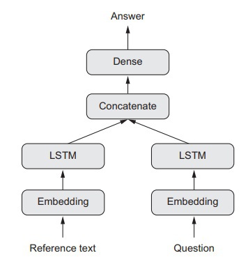
To understand this concept better, let’s talk about an actual multi-input model like the question-answering model. A question answering model has two input sources. These two inputs are;
- Question
- Text snippet
These two input sources collectively provide the model with the necessary information so that it can answer the question. The next plan of action for the model is to provide an answer to the question being posed. In a very plain and simple multi-input, the output is given in the form of an answer consisting of only a single word by utilizing a softmax function with a preloaded dictionary. The figure below depicts a question-answering model;
To build a multi-input question answering model by using a Functional API, we will need to define two input sources as independent branches. One branch will be responsible for encoding the text input, and the other will encode the question input. The data will be encoded into representation vectors, and these vectors will then be concatenated. Afterward, a softmax classifier will be on these representations. The code for doing this is as follows;
from keras.models import Model
from keras import layers
from keras import Input
text_vocabulary_size = 10000
question_vocabulary_size = 10000
answer_vocabulary_size = 500
text_input = Input(shape=(None,), dtype='int32', name='text')
embedded_text = layers.Embedding(
64, text_vocabulary_size)(text_input)
encoded_text = layers.LSTM(32)(embedded_text)
question_input = Input(shape=(None,),
dtype='int32',
name='question')
embedded_question = layers.Embedding(
32, question_vocabulary_size)(question_input)
encoded_question = layers.LSTM(16)(embedded_question)
concatenated = layers.concatenate([encoded_text, encoded_question],
axis=-1)
answer = layers.Dense(answer_vocabulary_size,
activation='softmax')(concatenated)
model = Model([text_input, question_input], answer)
model.compile(optimizer='rmsprop',
loss='categorical_crossentropy',
metrics=['acc'])
In regards to training this model, we can do so by either of the two approaches;
- Feeding the model inputs in the form of NumPy arrays lists.
- Feeding the model a dictionary that automatically maps the input names to the corresponding NumPy arrays (can only be done if you already named the inputs).
We will now demonstrate both of these approaches;
import numpy as np
num_samples = 1000
max_length = 100
text = np.random.randint(1, text_vocabulary_size,
size=(num_samples, max_length))
question = np.random.randint(1, question_vocabulary_size,
size=(num_samples, max_length))
answers = np.random.randint(0, 1,
size=(num_samples, answer_vocabulary_size))
model.fit([text, question], answers, epochs=10, batch_size=128)
model.fit({'text': text, 'question': question}, answers,
epochs=10, batch_size=128)
The first model.fit argument shows how you can feed a list of NumPy arrays as input and the last model.fit argument shows how you can feed a dictionary of inputs respectively.
Multi-Output Models
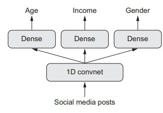
So far, we have talked about multi-input models, such as the question-answer model. Similarly, a functional API can also be used to construct a deep learning model that has multiple outputs, also referred to as heads. For instance, a multi-output model can be a deep learning model that analyzes the social media posts of an unknown person and give multiple predictions regarding the person’s age, profession, and gender, etc. These multiple predictions are, in essence, multiple outputs of the model.
Let’s see how a multi-output model of a maximum of three outputs can be built by using the functional API;
from keras import layers
from keras import Input
from keras.models import Model
vocabulary_size = 50000
num_income_groups = 10
posts_input = Input(shape=(None,), dtype='int32', name='posts')
embedded_posts = layers.Embedding(256, vocabulary_size)(posts_input)
x = layers.Conv1D(128, 5, activation='relu')(embedded_posts)
x = layers.MaxPooling1D(5)(x)
x = layers.Conv1D(256, 5, activation='relu')(x)
x = layers.Conv1D(256, 5, activation='relu')(x)
x = layers.MaxPooling1D(5)(x)
x = layers.Conv1D(256, 5, activation='relu')(x)
x = layers.Conv1D(256, 5, activation='relu')(x)
x = layers.GlobalMaxPooling1D()(x)
x = layers.Dense(128, activation='relu')(x)
age_prediction = layers.Dense(1, name='age')(x)
income_prediction = layers.Dense(num_income_groups,
activation='softmax',
name='income')(x)
gender_prediction = layers.Dense(1, activation='sigmoid', name='gender')(x)
model = Model(posts_input,
[age_prediction, income_prediction, gender_prediction])
A figurative representation of this model is shown below;
In such deep learning models, we have to specify a different loss function for each corresponding output or the head of the network. Take the gender prediction output given by the model, for the Neural network; this is a binary classification task. At the same time, giving an age prediction output is a scalar regression task, and the training process is also entirely different. Hence the nature of the task being performed by the model is different for each head, and that is why each head requires a specific loss function. Moreover, a primary requirement of gradient descent is the minimizing of the scalar. To do this, we will have to merge these different losses into a singular value, and only then can we proceed to train the model.
The most straight-forward and simple approach towards combining the losses is just to sum them up and to do so, Keras gives us the option of using the lists or dictionary of the ‘compile’ function so that we can specify the multiple outputs to the corresponding object. Afterward, we take the loss values from the outputs and sum them up into one global loss value. This can be then minimized, and the model can be trained.
The two options through which we can compile the losses of the multi-output model are as follows;
model.compile(optimizer='rmsprop',
loss=['mse', 'categorical_crossentropy', 'binary_crossentropy'])
model.compile(optimizer='rmsprop',
loss={'age': 'mse',
'income': 'categorical_crossentropy',
'gender': 'binary_crossentropy'})
The latter is only possible if you have tagged the output layers with specific names.
A very important thing to note regarding losses in a multi-output model is that if there is an imbalance loss contribution, the representations of the deep learning model will inherently be optimized for the task that has the current biggest individual loss value. This optimization comes at the expense of other tasks. We can avoid this by taking the multiple loss values and assigning each value with a level of importance, which defines its contribution to the global loss value.
The following lines of code show the loss weighting option in the compilation of a multi-output model;
model.compile(optimizer='rmsprop',
loss=['mse', 'categorical_crossentropy', 'binary_crossentropy'],
loss_weights=[0.25, 1., 10.])
model.compile(optimizer='rmsprop',
loss={'age': 'mse',
'income': 'categorical_crossentropy',
'gender': 'binary_crossentropy'},
loss_weights={'age': 0.25,
'income': 1.,
'gender': 10.})
To train the model, we can use the same two approaches defined for multi-input models, i.e; using a list of NumPy arrays or using a dictionary of NumPy arrays;
model.fit(posts, [age_targets, income_targets, gender_targets],
epochs=10, batch_size=64)
model.fit(posts, {'age': age_targets,
'income': income_targets,
'gender': gender_targets},
epochs=10, batch_size=64)
The latter is only possible if you have tagged the output layers with specific names.
Directed Acyclic Graphs of Layers
Apart from being used as the gateway for building models that have multiple inputs and multiple outputs, the functional API is also capable of allowing the user to implement neural networks that feature a complex internal topology. This makes the full use of Keras’s ability to support arbitrary neural networks. Moreover, the conceptual foundation of such a network is “acyclic,” meaning that no tensor will become the input of the layer that generated it.
The two notable neural network components which are implemented as graphs are;
- Inception Modules
- Residual connections
Understanding these two components is key to learning how we can implement a functional API to build a graph of layers.
Inception Modules
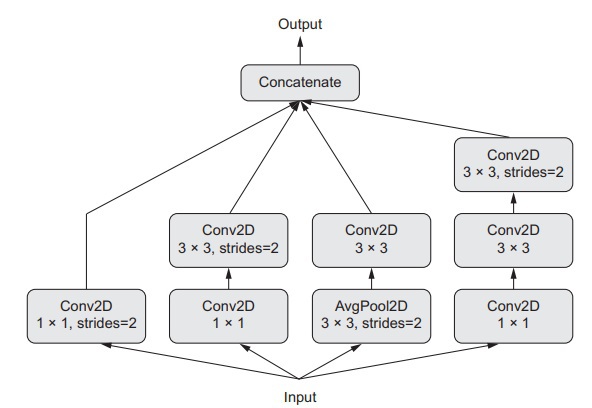
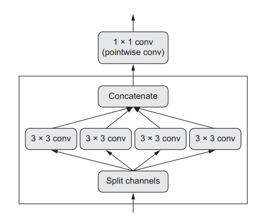
Inception is actually a network architecture which is chiefly used in convolutional neural networks. The architecture is made up of a stack of modules that break into several parallel branches. A basic setup of an inception module is as follows;
- Three or four branches, beginning with 1x1 convolution.
- Following up with a 3x3 convolution.
- Finishing with the result, which is an overall concatenation of the results accumulated from the convolutions.
The setup described enables the neural network to learn the two features; spatial and channel-wise features in a separate manner; this is way more efficient for the network rather than learning these features jointly. An inception module can be set up to be even more complex by adding in some pooling operations, making the sizes of the convolutions different, and using branches that do not have a spatial convolution. The figure below shows a module that has been taken from the Inception V3 model;
To implement this module, we will use a functional API and assume that there is an input tensor ‘x,’ which is a 4D tensor. The following lines of code demonstrate this assumption;
from keras import layers
branch_a = layers.Conv2D(128, 1,
activation='relu', strides=2)(x)
branch_b = layers.Conv2D(128, 1, activation='relu')(x)
branch_b = layers.Conv2D(128, 3, activation='relu', strides=2)(branch_b)
branch_c = layers.AveragePooling2D(3, strides=2)(x)
branch_c = layers.Conv2D(128, 3, activation='relu')(branch_c)
branch_d = layers.Conv2D(128, 1, activation='relu')(x)
branch_d = layers.Conv2D(128, 3, activation='relu')(branch_d)
branch_d = layers.Conv2D(128, 3, activation='relu', strides=2)(branch_d)
output = layers.concatenate(
[branch_a, branch_b, branch_c, branch_d], axis=-1)
If you want to analyze this module even further, you can access the full architecture of the Inception V3 model in Keras by using the argument;
keras.applications.inception_v3.InceptionV3
This architecture includes pre-trained weights.
Residual Connections
Residual connections are basically one of the common components found in a graph-like network; for instance, in deep learning models such as Xception, residual connections can be found in the architecture of the network. This component is an effective solution to the most observed problems that are found in most large-scale deep learning models;
- Vanishing gradients
- Representational bottlenecks
In any model that features more than ten layers in its network architecture, residual connections can benefit the model in one way or the other.
Residual connections essentially function to give the layers easy access to the output of a layer preceding it. This output is taken as input by this layer easily because of residual connections. In other words, a residual connection creates shortcuts between the layers in a sequential model.
Let’s consider a network which has same sized feature maps and implement a residual connection. For its implementation, we will be using identity residual connections. Note that this demonstration has an assumption that there is a 4D input tensor ‘x’;
from keras import layers
x = ...
y = layers.Conv2D(128, 3, activation='relu', padding='same')(x)
y = layers.Conv2D(128, 3, activation='relu', padding='same')(y)
y = layers.Conv2D(128, 3, activation='relu', padding='same')(y)
y = layers.add([y, x])
The above lines of code is for using residual connections with feature maps that are of the same size. A residual connection can also be implemented in a network when the feature maps are of different sizes, for such a case we simply use linear residual connection instead of identity;
from keras import layers
x = ...
y = layers.Conv2D(128, 3, activation='relu', padding='same')(x)
y = layers.Conv2D(128, 3, activation='relu', padding='same')(y)
y = layers.MaxPooling2D(2, strides=2)(y)
residual = layers.Conv2D(128, 1, strides=2, padding='same')(x)
y = layers.add([y, residual])
Layer Weight Sharing
Another one of functional API’s notable features is layer weight sharing. This basically refers to the API’s ability to reusing a certain layer many times. This is evident when we proceed to call on a layer two times. Normally, we would instantiate the layer on each call; however, in this case, we call on them without instantiating, and this results in the usage of the same weights on each call. By doing this, we can construct deep learning models that shared branches.
Let’s make this concept even more clear by discussing an example. Let’s say we have a model that is given a task to identify the similarity between two sentences in terms of semantics. In such a scenario, the model is dealing with two inputs, and the output is given either 0 or 1, meaning unrelated sentences and identical or reformulated sentences, respectively. In such a setup, the two inputs we are dealing with are interchangeable because the semantic relationship of sentences is commutative. Hence we do not need to build two separate models for dealing with the processing of each of these two inputs. In such a case, we would use a single layer to process both of these inputs, and this layer would be the LTSM layer. The representations of the LTSM layers are learned while taking both of the inputs into consideration. This is also known as the “Siamese LTSM model” or a “Shared LTSL model.”
The following lines of code detail how you can implement such a model using functional API;
from keras import layers
from keras import Input
from keras.models import Model
lstm = layers.LSTM(32)
left_input = Input(shape=(None, 128))
left_output = lstm(left_input)
right_input = Input(shape=(None, 128))
right_output = lstm(right_input)
merged = layers.concatenate([left_output, right_output], axis=-1)
predictions = layers.Dense(1, activation='sigmoid')(merged)
model = Model([left_input, right_input], predictions)
model.fit([left_data, right_data], targets)
Using Models as Layers
Another ability of the functional API is allowing models to be effectively used as layers, as is in the case for sequential and model classes. Consequently, we can use an input tensor and call on a model, in turn, receiving an output tensor. This can be done by using the following argument;
If the model we are using as a layer itself has several inputs and outputs tensors, then the method to call such a model should be through a list of tensors as shown below;
Similar to when we call an instance of a layer, calling upon an instance of a model uses the same weights the model has been trained upon. In other words, no matter if we call upon a layer or a model, the representations will remain the same and can be reused.
An example of what we can do by reusing a model is building a ‘vision’ model. This model has two inputs by using a dual camera as its source. To process the data coming from the two cameras, we don’t need to build two separate models and then merge them later on. A simple stream of data like this can be easily handled by using a low-tier processing technique, such as using layers that have them weights and representations. To implement a Siamese vision model, follow the lines of code shown below;
from keras import layers
from keras import applications
from keras import Input
xception_base = applications.Xception(weights=None,
include_top=False)
left_input = Input(shape=(250, 250, 3))
right_input = Input(shape=(250, 250, 3))
left_features = xception_base(left_input)
right_input = xception_base(right_input)
merged_features = layers.concatenate(
[left_features, right_input], axis=-1)
Inspection of Deep Learning Models Using Keras Callbacks and Tensorboards
This section will primarily focus on the ways through which we can better control the processes within our deep learning model and access its components more easily. In other words, we will explore the ways that will help us manipulate deep learning models more effectively. The reason why this is important is because when training deep learning models on large datasets with many epochs, we mainly use the model.fit() and model.fit_generator() arguments to control it. However, beyond the initial impulse, we do not have any control over the model, and hence, it is impossible always to avoid bad outcomes. The techniques detailed in this section will turn this model.fit() argument from a passively uncontrollable mechanism to a useful and autonomously smart enough argument that can deter bad outcomes
Using Callbacks to Act on an In-Training Model
Training a model is never a predictable process. We do not know how many epochs are needed for an optimal validation loss beforehand; we can only come to know after some trial and error. So far, we have practiced the approach of training the model just before it beings overfitting by plotting the validation and loss data to determine the number of epochs required to do so. This approach is inefficient and takes up a lot of resources.
So, an alternative to this approach is that instead of completing the entire training process to find out where the overfitting begins, we can just stop the training at the point where the validation loss values no longer show any improvement, saving us a lot of time and effort. To do this, we will need to use the Keras callback. Callbacks are basically objects which are given to the fit argument. The deep learning model then calls upon this object at different points during the training process. The features which make a callback so useful are;
- They have access to data which details the information regarding the model’s current state and performance
- It has the authorization of acting according to the situation, such as stop the training, save the model’s current state, bring in some other set of weights for the model to use, or even change the current state of the deep learning model.
Keeping these features of a callback in mind, we can use it for the following purposes;
-
As Checkpoints
, as a callback, has the capability of saving a model’s current state by simply saving its current weight set, it can make frequent saves giving us a checkpoint to revert the model if something goes wrong.
-
Premature Interruption
; a callback can step in and stop the training process of the model. This can be used for stopping the training of the model as soon as the improvement of the validation loss becomes stagnant.
-
Dynamic Adjustment
; a callback can change the values of certain parameters during the training process to make necessary adjustments, for instance, adjusting the learning rate of the optimizer during the network’s training.
- Remember the Keras bar? This is a practical implementation of a callback as it can log data and visualize representations.
Here’s a list of callbacks that are included in the keras.callback
module;
keras.callbacks.ModelCheckpoint
keras.callbacks.EarlyStopping
keras.callbacks.LearningRateScheduler
keras.callbacks.ReduceLROnPlateau
keras.callbacks.CSVLogger
We will just explain only a select few of these different callbacks.
The ModelCheckpoint and EarlyStopping Callbacks
The primary purpose of the EarlyStopping callback is to make the approach of achieving optimal validation loss, viable. In essence, we define a metric for the callback to monitor during the training. As soon as it detects that the metric value has reached its optimal point and can no longer improve, then it immediately interrupts the training. The EarlyStopping callback is commonly used in pairs with the ModelCheckpoint callback, the latter basically creating saved model checkpoints.
To understand these two callbacks better, let’s see how they are implemented in code;
import keras
callbacks_list = [
keras.callbacks.EarlyStopping(
monitor='acc',
patience=1,
),
keras.callbacks.ModelCheckpoint(
filepath='my_model.h5',
monitor='val_loss',
save_best_only=True,
)
]
model.compile(optimizer='rmsprop',
loss='binary_crossentropy',
metrics=['acc'])
model.fit(x, y,
epochs=10,
batch_size=32,
callbacks=callbacks_list,
validation_data=(x_val, y_val))
The ReduceLROnPlateau Callback
A common use of this callback is to reduce the model’s rate of learning when it detects that the metric being monitored, in this case, the validation loss, has stagnated in terms of improvement. This sets up for a very effective strategy of escaping the in-training local minima as we can control the learning rate in a loss plateau. Here’s an example of how we can use this callback;
callbacks_list = [
keras.callbacks.ReduceLROnPlateau(
monitor='val_loss'
factor=0.1,
patience=10,
)
]
model.fit(x, y,
epochs=10,
batch_size=32,
callbacks=callbacks_list,
validation_data=(x_val, y_val))
Writing a Custom Callback
If you’re looking for a callback that can do a specific function but can’t find one in the Keras’ list of callbacks, then you can just create a custom callback specifically for your purpose. A callback is basically implemented in a network by simply sub-classing the keras.callbacks.Callback class. A callback can be implemented at any point in the training by using these prenamed methods;
- on_epoch_begin; gets called on at the start of every iterating epoch
- on_epoch_end; gets called on at the end of every iterating epoch
- on_batch_begin; gets called on just before each batch’s processing
- on_batch_end; gets called on as soon as the processing of a batch is finished
- on_train_beign; gets called on at the start of the training
- on_training_end; gets called on at the end of the training
All of these methods, which are listed above, are called along with a logs
argument (a dictionary that has data about the preceding batch, epoch, or training iteration).
Moreover, the two attributes listed below are easily accessible by a callback;
- self.model; the instance of the deep learning model from where the callback is being called upon.
- self.validation_data; the value of the validation data, which was passed onto the fit argument.
Let’s look at the following example of a custom-made callback. This callback takes the activation values of the layers at the end of every epoch and saves them on a disk as NumPy arrays;
import keras
import numpy as np
class ActivationLogger(keras.callbacks.Callback):
def set_model(self, model):
self.model = model
layer_outputs = [layer.output for layer in model.layers]
self.activations_model = keras.models.Model(model.input,
layer_outputs)
def on_epoch_end(self, epoch, logs=None):
if self.validation_data is None:
raise RuntimeError('Requires validation_data.')
validation_sample = self.validation_data[0][0:1]
activations = self.activations_model.predict(validation_sample)
f = open('activations_at_epoch_' + str(epoch) + '.npz', 'w')
np.savez(f, activations)
f.close()
With regards to conceptual knowledge to use callbacks, up until now we have covered it, the remaining details are basically technical details and you can look them up easily.
Tensorboard: The TensorFlow Visualization Network
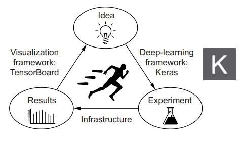
The key element in building an effective deep learning model for any experiment is to be aware of the internal situation of the model’s current state. Moreover, this is the exact purpose of experiments, which is to find out how effective is the deep learning model at handling the information and performing the required tasks. Similarly, a model’s improvement is an iterative process, not a defined process that you architect it one time, and it turns out to be either good or bad. Instead, you come up with an idea; you build a suitable experiment to test that idea. You perform this experiment and check the resulting information you obtain, and from this, you get another idea and repeat the process. In this way, you iterate this entire process and refine your deep learning model with even more powerful and effective ideas being the foundation of the model. The reason we discussed this topic is because of the role the Tensorboard plays here; it basically fulfills the job of processing the experimental results in this iterative process.
A TensorBoard is a visualization tool that comes prepackaged in the Keras framework, and this tool is browser-based. However, this tool is only accessible if the deep learning model is using the Keras framework along with a TensorFlow backend engine. Tensorboards are mainly used for displaying what is actually happening in the model during the training session.
Furthermore, using the Tensorboard to monitor several other metrics apart from the validation loss will provide a better insight into how your model is working and a better understanding of how it can be improved. Tensorboard gives convenient access right on the browser to several features such as;
- Displaying visualizations of the in-training metrics to monitor them.
- Displaying the makeup of the deep learning model.
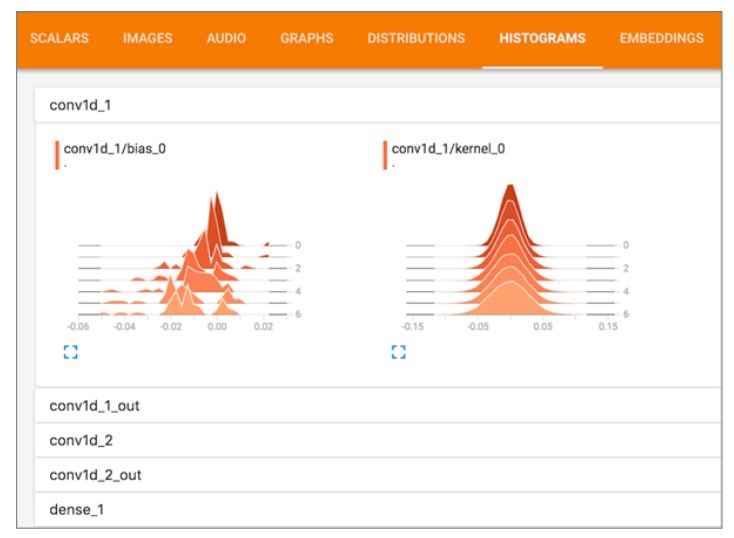
- Displaying both the activation and gradient histograms.
- 3D surveying the embeddings.
Lets put these features to use in a 1D convnet being trained on the IMDB sentiment analysis task.
The makeup of the deep learning model will be primarily to make the word embeddings visualizations more tractable. ;
import keras
from keras import layers
from keras.datasets import imdb
from keras.preprocessing import sequence
max_features = 2000
max_len = 500
(x_train, y_train), (x_test, y_test) = imdb.load_data(num_words=max_features)
x_train = sequence.pad_sequences(x_train, maxlen=max_len)
x_test = sequence.pad_sequences(x_test, maxlen=max_len)
model = keras.models.Sequential()
model.add(layers.Embedding(max_features, 128,
input_length=max_len,
name='embed'))
model.add(layers.Conv1D(32, 7, activation='relu'))
model.add(layers.MaxPooling1D(5))
model.add(layers.Conv1D(32, 7, activation='relu'))
model.add(layers.GlobalMaxPooling1D())
model.add(layers.Dense(1))
model.summary()
model.compile(optimizer='rmsprop',
loss='binary_crossentropy',
metrics=['acc'])
Before we can start using the Tensorboard, we first need to define a directory for it to store the log files generated by the Tensorboard;
We will now begin the training for the model by using the Tensorboard
callback. The purpose of this callback is to take the log event files generated and save them at the specified directory on the disk.
callbacks = [
keras.callbacks.TensorBoard(
log_dir='my_log_dir',
histogram_freq=1,
embeddings_freq=1,
)
]
history = model.fit(x_train, y_train,
epochs=20,
batch_size=128,
validation_split=0.2,
callbacks=callbacks)
If you have installed the TensorFlow backend engine, then the tensorboard
utility has also been automatically installed on your system. We can now proceed to open the Tensorboard utility by using the command line.
$ tensorboard --logdir=my_log_dir
To see the visualized training session of the deep learning model, open the browser and enter the address;
http://localhost:6006
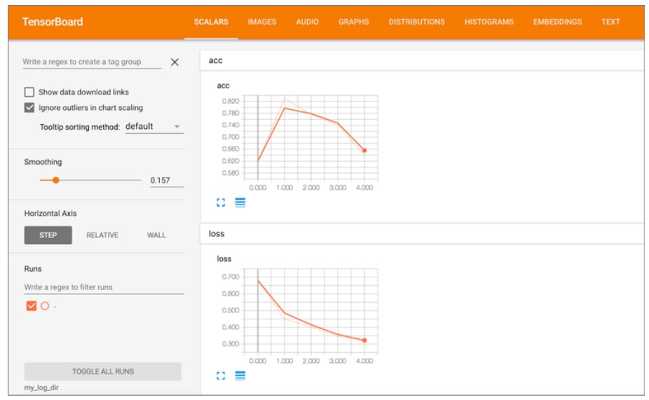
You can see all kinds of useful metric visualizations and other stuff as shown in the figures below;
(Tensorboard Metric Monitoring)
(Tensorboard Visualizing the Activation of Histograms)
If we go the embeddings tab in the Tensorboard, we can easily analyze the attributes of the ten thousand word vocabulary input of our model such as;
- Embedding locations
- Spatial relationships
One more point to note is that originally, the embedding space is of a higher dimension, i.e., 128-dimensional. To visualize and display it, the Tensorboard reduces the dimensional size down to either 2D or 3D. This is done by using algorithms such as the ‘dimensionality-reduction.’
Moreover, you can choose which dimensionality reduction algorithm you want to use as the Tensorboard offers two choices in this regard, namely the PCA (Principal Component Analysis) or the t-SNE (t-distributed Stochastic Neighbor Encoding). In the figure below, we can see a visualization of the embedding space of the words with positive and negative connotations.
Just as how we accessed to useful information by going to the embedding tab in the Tesnorboard, you can explore the other tabs and see what kind of information they have to offer.
Working with Advanced Methods and Getting Optimized Results
Most of the time, programmers tend to try out various deep learning models without using any proper techniques or methods just to find something that simply works. In this section, we will explore the advanced methods, which are essentially the building blocks or the foundation of making amazing and effective deep learning models.
The Advanced Architecture Patterns
In the preceding sections, we explored a very important and effective network architecture for building competitive deep learning models, and this design pattern is the ‘residual connections.’ Apart from this pattern, we will discuss two more architecture patterns, namely;
-
Normalization
-
Depthwise separable convolution
Although these architecture patterns are also commonly found in good deep learning models, they basically set up the foundation for a flagship tier deep learning convnets.
Batch Normalization
Normalization does not refer to one specific pattern or method. Instead, it covers a broad range of methods. However, the goal of these methods is essentially the same, i.e., to normalize the various samples being inputted into the deep learning model. In other words, it takes different samples and converts them into similar samples for the model to train on. In this way, the model copes well when dealing with new data and generalizing predictions effectively and accordingly.
Out of this broad category of methods, the most common normalization method we have seen being used not only in the examples demonstrated in this book but also in some exemplary deep learning models as well and this normalization method is the one where we consider a data sample and take out the mean value from the data, hence centering it on 0. Afterward, we equip this data with a ‘unit standard deviation,’ and this is obtained by simply taking the standard deviation and dividing the data on it. The result is an assumption that considers the data to now be following a gaussian distribution (a normal distribution) while being centered and scaled to unit variance.
normalized_data = (data - np.mean(data, axis=...)) / np.std(data, axis=...)
Previously, we saw that the examples using normalization would only feed the data to the network only after it had been normalized. However, for it to be more effective, data normalization should be done after every transformation that is functioned by the neural network.
Batch normalization is essentially a type of layer in Keras (BatchNormalization
) that can adapt to the shifting mean and variance attributes during the training session and manage to normalize the data even then. Its working is basically dependant on being the maintainer of a steady exponential moving average of the two internal metrics; the mean (according to each batch) and the data being learned during training’s variance. The primary goal of a batch normalizer is similar to the residual connections in the sense that batch normalization tends to facilitate the gradient propagation, making it possible to build even deeper neural networks for a model. Similarly, certain phenomenally deep neural networks can only go through training if there are several BatchNormalization
layers present. Otherwise, it cannot be trained. We also see the use of this batch normalization layers in the architectures of the popular advanced convnets such as ResNet50, Inception V3, and Xception.
Usually, a BatchNormalization
layer is implemented in such a way that it either succeeds a convolutional layer or a densely connected layer as shown below;
conv_model.add(layers.Conv2D(32, 3, activation='relu'))
conv_model.add(layers.BatchNormalization())
dense_model.add(layers.Dense(32, activation='relu'))
dense_model.add(layers.BatchNormalization())
From the lines of code, you can see that the first one shows a batch normalization layer coming after a convolutional layer and the second shows it coming after a desenly connected layer.
Furthermore, this normalization layer identifies and specifies the feature axis to be normalized by using the axis
argument with a default value set to -1 (this value refers to the very last layer in the input tensor). This specific value is accurate for using after layers after the following layers; ‘Dense’ layers, ‘Conv1D’ layers, ‘RNN’ layers, and ‘Conv2D’ layers (with a pre-requisite that the argument data_format is specified to “channels_last”). However, when using this normalization layer in niche cases, the axis argument’s value is set to 1 instead of -1. In this case, the data_format argument of the Conv2D layers should be inverted, i.e., set to “channels_first.”
Depthwise Separable Convolution
In topic, we will explore a unique layer that, when added to a network by replacing the convolutional layer Conv2D, can not only improve the speed of the network in which it is being used but also make it several degrees lighter. The network becomes faster because are now lesser floating-point operations, and it becomes lighter as there now is a smaller set of trainable weight parameters, making it perform better by several percentages on specific tasks. A layer with such properties is none other than the depthwise separable convolution layer, also known as SeperableConv2D.
The way this layer operates is that it takes each independent channel of the input and executes spatial convolution on each of the corresponding channels preceding the use of pointwise convolution to mix the output channels (essentially a 1x1 convolution). This process is the alternative equivalent of segregating two features - the spatial and channel-wise features. This step is sensible under the assumption that although the spatial locations are intricately correlated in the input, the varying channels remain independent. This ultimately results in a lighter requirement for the network to use fewer representations and learn better, perform convolutions and ultimately, resulting in a high-performance deep learning model by hardly requiring any parameters and even involving a lesser number of computations, making up a model that is small yet speedy.
(A Depthwise Convolution Followed by a Pointwise Convolution)
The usability, effectiveness, and importance of this convolution layer become evident when we are working with small models and training on them from the ground up on a limited amount of data. To understand depthwise separable convolutional layers even better, let’s see a demonstration of how a lightweight deep learning model can be built by using a depthwise separable convnet and train it for the task of image-classification (in essence, softmax categorical classification) on a limited dataset;
from keras.models import Sequential, Model
from keras import layers
height = 64
width = 64
channels = 3
num_classes = 10
model = Sequential()
model.add(layers.SeparableConv2D(32, 3,
activation='relu',
input_shape=(height, width, channels,)))
model.add(layers.SeparableConv2D(64, 3, activation='relu'))
model.add(layers.MaxPooling2D(2))
model.add(layers.SeparableConv2D(64, 3, activation='relu'))
model.add(layers.SeparableConv2D(128, 3, activation='relu'))
model.add(layers.MaxPooling2D(2))
model.add(layers.SeparableConv2D(64, 3, activation='relu'))
model.add(layers.SeparableConv2D(128, 3, activation='relu'))
model.add(layers.GlobalAveragePooling2D())
model.add(layers.Dense(32, activation='relu'))
model.add(layers.Dense(num_classes, activation='softmax'))
model.compile(optimizer='rmsprop', loss='categorical_crossentropy')
Depthwise separable convolutional layers are not exclusive to being only used in small deep learning models. On the contrary, the depthwise convolutions are also the building blocks network architectures for large scale deep learning models such as the Xception model, a high-speed convnet that can be accessed through the Keras framework as it comes pre-packaged in it.
Hyperparameter Optimization
The process of building a deep learning model and architecting a neural network usually involves arbitrary decisions and guess-work. For example, you might ask yourself how many stack layers does the model need, what’s the optimum number of units and filters for each layer I am using? You might find yourself choosing between a relu activation or some other function for the best result, the decision of either using a BatchNormalization
layer or not or even the number of dropouts you should use and this list continues. All of these parameters, you are pondering on come under the category of “Hyperparameters.” The reason why they are termed as such is for avoiding confusion between these architecture-level parameters and a model’s parameters that are trained using backpropagation.
Architecting a good neural network can be done by intuition, and such intuition can only be developed by repeated practice and experience. This leads to the development of skills for hyperparameter tuning.
However, there are no set rules for doing this. If we want to push our model to its very limits and get the most out of it, we cannot settle for arbitrary choices defining our deep learning model as human choices are always subject to fallacy and error in one way or the other. In other words, even if a person ends up developing a commendable intuition, in the end, the initial decision will always end up being sub-optimal. In such a scenario, the engineers and researchers of machine learning will have to grind their time in repeatedly improving their deep learning model. At the end of the day, the task of tweaking the hyperparameters to optimize them is not suitable for humans and is best left to machines themselves.
In short, the jobs we should spend our time perfecting is the exploration of the realm of possible decisions in a systematic and principled way. To do so, we are required to scavenge through the network’s architecture and look for the most optimally functioning space empirically. This is the essence and core of hyperparameter optimization, a critical and effective field of research. A typical hyperparameter optimization procedure is as follows;
-
Automating the nomination of a hyperparameter.
-
Constructing the deep learning model accordingly.
-
Proceeding to fit these parameters to the input training data and calculating the model’s performance on the corresponding validation dataset.
-
Automating the nomination of another set of hyperparameters for the model to try out.
-
Repeating steps 2 and 3.
-
Gradually moving on to analyzing the model’s performance on the testing dataset.
The key to performing the hyperparameter optimization process successfully is twofold:
-
The algorithm is not responsible for nominating the sets of hyperparameters for the model to try
-
Careful consideration is given to the historical validation performance for the different hyperparameters sets used so far.
As such, there are several techniques available to use, such as Bayesian optimization, genetic algorithms, simple random search, etc.
Training the model’s weight is comparatively easy and simple. All you have to do is just calculate the loss functions on the current mini-batch data and use the backpropagation algorithm so that you can push these weights in the right direction. On the other hand, updating a hyperparameter is anything but easy. To understand this, try to analyze these two situations;
-
It can be expensive in resource terms to calculate a feedback signal to determine whether the current set of hyperparameters creates an optimal model for the task at hand. This means that it will require the machine learning engineer to repeatedly build and train new models from the ground up on the given dataset.
-
A hyperparameter space is essentially a network of discrete decisions. This means that it cannot be differentiable or continuous. Due to this, the gradient descent optimization is not an option for use with a hyperparameter space. Hence, we are left with using optimization methods and techniques that are gradient-free, and these techniques are inefficient as compared to gradient descent.
Due to the great difficulty of these challenges being faced by machine learning engineers while the field is relatively is young and not well-explored, we are stuck with using only a limited set of tools to optimize deep learning models with. Most of the time, random search becomes the only viable option. However, it is a very naïve technique as we are essentially choosing random hyperparameters to try out and keep on repeating this process. However, a tool more reliable than random search and can perform arguably better than it is a Python library for hyperparameter optimization that predicts a set of hyperparameters likely to be optimal for the model by using Parzen estimators is the Hyperopt
tool and this tool can be accessed from;
https://github.com/hyperopt/hyperopt
In Keras deep learning models, there is a similar tool that essentially integrates Hyperopt so that they can be used with deep learning models using Keras and this library is known as Hyperas
and can be accessed from;
https://github.com/maxpumperla/hyperas
In short, hyperparameter optimization is an essential and very important tool for building top tier and high-performance deep learning models.
Model Ensembling
The last technique we will be discussing for this book is the model ensembling, a robust tool that can bring out the maximum potential of your deep learning model. Model ensembling involves taking the predictions of different models and pooling them to produce an overall better prediction.
The core idea of model ensembling that all the good models are designed to be optimal in their own ways. For example, each of them looks at a certain aspect of the data to give good predictions, by combining these predictions looking at different aspects together, we can produce an even better prediction that includes all these different aspects of the data. For example, let's look at a typical classification task. To ensemble the different sets of classifiers, we can just average their predictions by setting up a meantime;
preds_a = model_a.predict(x_val)
preds_b = model_b.predict(x_val)
preds_c = model_c.predict(x_val)
preds_d = model_d.predict(x_val)
final_preds = 0.25 * (preds_a + preds_b + preds_c + preds_d)
This is only viable if all the classifiers have more or less the same level of performance. If one is worse than the rest, the resulting prediction will be heavily affected.
A more efficient and optimal method of ensembling different classifiers is by performing a weighted average in such a way that good classifiers are given a heavier weight set, and bad classifiers are given low weight sets. To find an optimal set of ensembling weights, we can either use the random search or a simple optimization algorithm like the Nelder-Mead;
preds_a = model_a.predict(x_val)
preds_b = model_b.predict(x_val)
preds_c = model_c.predict(x_val)
preds_d = model_d.predict(x_val)
final_preds = 0.5 * preds_a + 0.25 * preds_b + 0.1 * preds_c + 0.15 * preds_d
The methods through which we can approach model ensembling is very diverse. However, the method shown above is seen to be a very strong foundation for performing a good model ensembling.