6
The Turbulent Human Brain: An MHD Approach to the MEG
6.1 Introduction
Among the currently available time-dependent functional imaging technologies for the human brain [1], the noninvasive magnetoencephalograph (MEG) is unique in providing excellent temporal resolution and good spatial resolution of cortical activity. The MEG signals are relatively insensitive to the boundaries of conductivity in the head, allowing for simple electromagnetic modeling of sources. MEG has been found useful in diverse function-related neuroanatomical source localizations. Some examples include brain tumors [2], epilepsy [3] [4], neurogenic pain [5], and affective priming [6]. MEG has also contributed to the characterization of brain states in response to psychopharmacological agents [7–9] and global brain disorders such as Down's syndrome [10], Alzheimer's disease [11], the Parkinson syndrome [12], and schizophrenia [13] [14]. MEG source imaging techniques, analogous to those reflecting brain activity involving oxygen and glucose brain energy utilization such as positron emission tomography (PET) and blood-oxygenation-level-dependent (BOLD) imaging, quantifies localized changes of source amplitude and power [15] [16].
Linear MEG signal analyses include methods making use of linear analyses, including the correlation functions and band-limited time–power–frequency spectra (e.g., the Stockwell transform) [17–19]. Nonlinear analyses of the MEG using measure theoretic approaches to dynamical systems have included a variety of entropies and characteristic dimension [20–23]. Most, if not all, MEG studies that have focused on localizing sources or characterizing fields have treated the MEG record as an implicitly epiphenomenal reflection of underlying electrophysiological events [24]. Source space analysis of the MEG signals use localization techniques such as the linearly constrained minimum variance (LCMV) beamformer (SAM, synthetic aperture magnetometry) to estimate the relevant electrical sources from the magnetic signal [25–27].
In these studies, we regard the MEG recording of magnetic signals as themselves, B = μH; where B is the magnetic flux density, μ is the magnetic permeability (of the material in a vacuum), and H is the magnetic field strength. Although the MEG is generally modeled using quasi-static electromagnetic equations, the signals are time varying and therefore are more accurately described by the Maxwell equations. It has been assumed that this correction is small enough, below frequencies of about 1 kHz, to be ignored. We minimize the emphasis on the inferred E field and its associated electrical currents, Ji, except when required by the magnetohydrodynamic, MHD approach's development. Deemphasizing E and Ji is almost similar to the treatment of generic B and E fields in space plasmas, in which the electrical field E (the curl of which is the magnetic field), conducts fast enough to outrun the slower, potentially information-bearing B field [28–30].
It is more typical in MHD magnetic induction and conservation equations to consider, relative to the E currents, the B field as “frozen in,” whereas our premises are different with respect to the temporal disparity. The MHD assumption is that the magnetic field may travel unchanged,  . Our fluctuating brain MEG data suggests something different. In this change in the usual MHD emphasis, the faster conducting E field has disappeared out of the frame and the B field is fluctuating as a time-dependent dynamical system.
We characterize the magnetic flows of the brain's B fields as dynamical systems in the context of MHD; the study of magnetic field dynamics in an electrically conducting fluid setting [31], which may involve aqueous solutions of electrolytes such as those found in the brain's interstitial and cerebrospinal fluids [32].
This orientation has led us to a set of new ideas concerning the potential information processing roles of both global and local brain magnetic field dynamics resembling those of MHD turbulence. Studies of 171 subjects' global resting MEG records have yielded evidence, through the use of multiple measures, for turbulent magnetic field dynamics. This includes possibilities for a pathophysiology and therapy involving dynamical entropy deficits [33]. A new combination of MEG source localization techniques [25] [34] and a new measure of topological/metric entropy, rank vector entropy (RVE) [35], has resulted in a localization technique using the RVE measure of complexity that appears more sensitive to neocortical dynamics than is simple power. The known informational richness of turbulent (chaotic) dynamics [36] [37] and the evidence for the existence of this state(s) in the human brain's local and global magnetic fields [38] [39] combine to suggest a new MHD field dynamic approach to MEG studies of human brain mechanisms and behavior. For example, might it be possible through frequency and nonlinear parameter optimization to configure a very weak external dynamical magnetic field in the pT range that would interact with the brain's intrinsic magnetic field directly (too weak for the induction of local electrical events), yielding increases or decreases in the brain's magnetic field dynamical entropy of potential therapeutic benefit.
6.2 Autonomous, Intermittent, Hierarchical Motions, from Brain Proteins Fluctuations to Emergent Magnetic Fields
Intuitively, outlining the spatial–temporal, anatomical–dynamical hierarchies [40] of the taskless, resting human neocortex in action, we imagine the neuronal intracellular structural and functional aqueous entropy-driven proteins in autonomous motion with a documented range of characteristic times from 104 to 10−12 s [41–43]; scaling (fractal) subthreshold ion channel membrane-conductance fluctuations [44]; a variety of intermittent single-neuron spike discharge patterns [45]; local and global neuronal network dynamics [46] including intermittent bursting and avalanches [47]; surrounding the network are the local E field potentials [48] [49]; and finally, the subject of this work, the dynamical patterns found in the brain's emergent magnetic fields [32]. Studies of the influence of weak fields on neuronal thresholds and activity [12–14] suggest a physiological role for “feedback fields” [50] in emergent E and B fields.
Analogous to the shift in focus from the particle to the field in quantum field theory, we move our attention from neuronal and neural network electrical sources to the dynamics found in attendant brain magnetic fields. Although dipolar and multipolar magnetic polarity have played a prominent role in linear static models of the MEG record [51–53], from the nonlinear graphical and measure point of view, magnetic field diffusivity leading to sharing and crossing of magnetic field lines and their apparently intrinsic stretch and fold dynamics (in R2) result in complicated fields. In these MEG studies of the task-free, “resting” human brain, we consider the behavior of the brain's magnetic field, B qua B, and not as an inferential, epiphenomenal reflection of the activity of its electrophysiological source [10]. A (necessarily) three-dimensional magnetic field in an electrical conducting fluid, such as the ionic interstitial fluid of the brain, behaves akin to an ensemble of differential material line elements that are being stretched and folded into turbulent flows [29]. It is usually represented graphically in R3 with the stretch in the x direction, fold in the y direction, and E field (via charge velocity ν)–B field shear in the z direction [54]. Dynamically, this stretch–fold–shear, SFS, mechanism operates in thin magnetic diffusive layers at the boundaries of repeating arrays of magnetic helical vortices (solenoidal flows) [55].
As noted earlier, a natural theoretical context for the examination of the behavior of human brain magnetic fields is MHD, particularly in light of our discovery that human brain magnetic fields are measure-theoretically turbulent [56]. Heisenberg's heuristic formulation of statistically isotropic and homogeneous hydrodynamic turbulence, his use of the physical mixing length of eddy viscosity, and energy (power) spectral functions [57] inspired Chandrasekhar to launch a dozen year (1949–1961) investigation of turbulent electrically conducting fluids in the presence of magnetic fields [58]. His initial finding was that Heisenberg's integral equations could be reduced to a linear first-order differential equation by a change in variables using wave number spectral representation, F(k), as the dependent variable and vorticity,  , curl of the flow velocity, as the independent variable. This led to his studies of convective dynamic instabilities in electrical conducting fields and MHD turbulence using techniques such as double and triple correlation tensors involving the interactions of charge velocity and the scalar intensity of magnetic fields. He used equations with eddy viscosity and electrical conductivity to elucidate dissipative energy exchanges between velocity and magnetic fields. His formulations of MHD turbulence included the recovery of the Kolmogorov inertial zone spectral scaling exponent of 5/3. Chandrasekhar can be said to have played a large part in creating the mathematical discipline of MHD.
6.3 Magnetic Field Induction and Turbulence; Its Maintenance, Decay, and Modulation
Using general vectorial field equations and their graphical representations, Figure 6.1 summarizes an MHD context for the dynamical analyses of the time dependent changes in human brain magnetic flux density, B. Figure 6.1a portrays the vectorial flow of the magnetic field generated by the flow of the impressed ionic current (and return current, not shown) via the dendritic tree of Cahal's classical pyramidal neuron, which lies orthonormal to the surface of the neocortex. We assume a charge velocity, ν, estimated to be 150 ms−1 [59], field strength of 2–4 mV mm−1 [50], and designate arbitrarily a current I  10−7 A, a free space permeability (ease of magnetization of the material) of μ0 = 4π × 10−7 and making measurement at distance r−3 (m). This leads to an estimate of the B field Faraday induction (Figure 6.1b,c) within the range of the human brain B fields we have observed experimentally using the MEG: B = μ0I/2πr ≈ 2 × 10⁻¹³ to−15 T ≈ (500–4000fT), Figure 6.1b,c [11] [13].
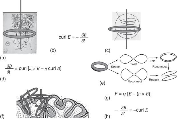
Figure 6.1 (a–h) Graphical and symbolic representations of the putative MHD of the neocortical magnetic fields.
As noted, the generic dynamical motions of turbulent field lines are the nonuniform stretch and fold mechanism [54] [60, 61]. It is responsible for increased “multifractal” magnetic flux density [62] and results from the nonaxiosymmetric, nonuniform mutual shear of electrical charge flow velocity, ν, and magnetic fields fluxes, B [30]. Magnetic field turbulent mixing arises from shear-induced, nonuniform stretching and folding of magnetic field lines, magnetic loop diffusivity engendered connections and their reconnections. This accompanies volume preserving folding and packing, thereby increasing the local magnetic flux density in regional B fields (Figure 6.1d,e), while not violating the conservation equations of MHD [58]. The vectorial direction of the traveling charges of pyramidal cell dendritic trees is orthogonal to the sulci and gyri of the neocortical surface. The transverse magnetic field B loops are generally parallel to the neocortical surface but they also become involved in its gyri and sulci corrugation-induced multidirectionality of E and B fields as shown (Figure 6.1f). It is of interest in this regard that recent studies of spatial order in neocortical pyramidal layers (layer V in mouse) have revealed that the repeating patterns of pyramidal cell “clusters” are arranged tangentially, a parallel orientation with the neocortical magnetic field [63]. Shear engendered eddy viscosity is minimal when the two fields are mutually transverse. Shear viscosity is maximal (and B is better maintained against dissipative loss) when E and B fields are aligned. In astrophysical contexts, magnetic-field-aligned currents are called Birkeland currents [64]. Evolutionarily (say from chicken to man), the increasing corrugation of the neocortical surface increases sheer when E and B fields are parallel (Figure 6.1f). This contributes further to magnetic field line diffusivity, crossings, and turbulence in the MEG signal.
Another contribution to the turbulent mixing of the B field is the Lorentz force, F, on a point charge, q, with instantaneous velocity, ν. Along with its electric E, and magnetic B fields, F is given by equation, Figure 6.1g. It is similar to a modulating “feedback” term in the electromagnetic system. Of particular interest here is what some call the Lorentz or magnetic force = qv × B [65]. In Figure 6.1h, the Lorentz force field reversal of the induction equation, Figure 6.1b, is the (“left-hand rule”) Lenz electromagnetic version of the Newtonian conservation of energy law. Currents arising from a magnetic flux engender a magnetic flux with its curl counter in field direction to the original current [65]. There cannot be an infinite regress of increasing magnetic energy. On the other hand, a possible net B field yield is possible in turbulent MHD in which the presence of turbulence is equivalent to the presence of a magnetic dynamo. This is clearest in the context of the kinetic dynamo problem, transient dynamos have been found to be theoretically and experimentally possible in nonaxiosymmetric, three-dimensional MHD turbulent systems with a relatively large charge ν [28]. The graphics and equations of Figure 6.1 serve as frameworks for the following ergodic measure theoretic, statistical studies of human brain MHD turbulence. In this context, we study magnetic field “resting” human MEG data [14] [66] and their statistical characterizations using quantities from ergodic measure theory [37] [67–69] to test the hypothesis that the taskless human brain magnetic fields are intrinsically turbulent.
In the interest of examining time-dependent, spatially extended human brain magnetic field activity, we study time series of the spatial derivatives of B field, ∂B/∂l where l is the distance between symmetrically placed MEG sensors constituting a symmetric sensor differences series, ssds. The values ranged between 10−15 and 10−13 T, ≈ 50–4000 fT) as recorded from pairs of centrally located MEG sensors; in these studies, the difference [C16(L) − C16(R)] constitutes the ssdsi. The use of ssds exploits the approximate hemispheric symmetry of the human brain [70] by quantifying the asymmetry, the nonaxiosymmetry, required to avoid magnetic field cancellations and allowing the observations of turbulence-related (“dynamo-like”) dynamics [28] [71]. The ssds transformation serves several purposes: (i) it includes a turbulent spatial-derivative parameter over time; (ii) imposes a local gauge, [(0-ssds max) fT/ ; (iii) serves as a time traveling, local regularized comparison; (iv) reduces the penetrance of electromagnetic field correlates of blink, cough, and movement as well as the cardiac and respiratory signals that both symmetric sensors generally share; (v) tends to cancel the symmetrically shared MEG (and electroencephalography (EEG)) Δ, θ, α, β, γ modes. In their place, we find the dynamics in the scaling, similarity regime [72]; (vi) is similar to the difference over space of the paired velocity probes used in experimental hydrodynamic turbulence studies; and (vii) minimizes central values and emphasizes higher moments and outliers, an effect facilitating the quantitative description of the dynamical and statistical properties of turbulent intermittency [73] [74].
Figure 6.2 represents the spatial sensitivity profile of a single central pair difference recording, the single ssds = [C23(L)–C23(R)] in which the difference is considered a single differential sensor, that is, the planar gradient,  , of the normal field. Note that the lighter colored portion of the graphs include a significant portion of the three-dimensional region including neocortical layers II and III in central, parietal, frontal, and some temporal areas. The techniques similar to that used here, of the paired sensor difference series, ssds(i), have been used to reduce or remove the mean and double or more the higher moments in analyses of nonstationary neural membrane conductance noise [73–75].
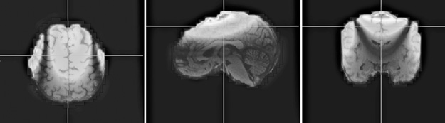
Figure 6.2 In lighter color, the neocortical magnetic field r > 0.70 correlated with the activity of the single sensor pair difference, [C23(L) − C23(R)] = ssds.
Figure 6.2 illustrates (on the same subject's magnetic resonance imaging (MRI) the MEG-correlated voxels from a single C16, ssds pair difference recording seen in the axial, sagittal, and coronal planes. Lighter areas indicate the voxel neocortical volume to which the red C23 sensor pair's ssds is (r > 0.70) correlated. The single (one pair difference) ssds sensor (in red) appears to capture much of the magnetic neocortical surface we study in the central brain's global B field dynamics.
The B field pair difference is a field property (∂B/∂l) with a centimeter length scale) being naturally equipped with a tangential gradient, in our studies (with the exception of Figure 6.2)  [C16(L) − C16(R)] = ssds. This spatial derivative is the primary time-dependent data in our studies of the properties of the MEG magnetic field time series. In constructing and using measures on ssds, we recall Ornstein's theorem, using isomorphism in measure as criteria, says there was only 1 equiv measure on expanding, mixing dynamical systems, its entropy [76] [77]. If one were to inquire further as to how the entropy should be computed, the answer (as of now) would be that there is no single method. In its place, there are many measure-theoretic equivalent ones [78]. Our effort to make this estimation has been to use multiple (each acknowledged as incomplete) measures, simultaneously noting the patterns among their values relative to those of other measures and patterns of relative changes among them [79–82]. With respect to changing relationships between measures, a robust example is the variably inverse relationship between topological entropy, hT, and the scaling exponent α, the slope of the middle third of the log–log plot of the frequency (power) spectral transformation [32].
Measures are computed on the time-dependent behavior of orbits embedded in n-dimensional phase space. This corresponds to tracking the smooth ssds orbital visits to available “states” or “configurations.” Phase space orbits are typically graphed in dimension Rn, with values corresponding to those at time t, time t − 1…t – n, as in Figure 6.3, in which n = 3. Most of the mathematical foundations of ergodic invariant measures to be used in an examination of these phase portraits has been established in the settings of well-defined, uniformly hyperbolic (expanding, contracting, mixing) statistically stationary states such as Axiom A diffeomorphisms [76] [83] that have Gaussian statistics. Real human brain magnetic field data, similar to hydrodynamic turbulence itself, is nonstationary, nonuniform, and prominent as the dynamic that has made for the most difficulty in mathematical hydrodynamic theory, intermittency [84–86]. Its statistics tend to have nonfinite variance. It is also the case that intermittency is a dominant dynamical pattern at many levels of observation in time series of brain function, from bursting in membrane conductance and neuronal spike trains [87], neuronal avalanches [47], local field potentials (LFPs), and regional and more global magnetic fields [32] [88, 89]. Intermittency in paired velocity-probe-difference time series is characteristic of hydrodynamic and MHD turbulence [36] [84, 90].
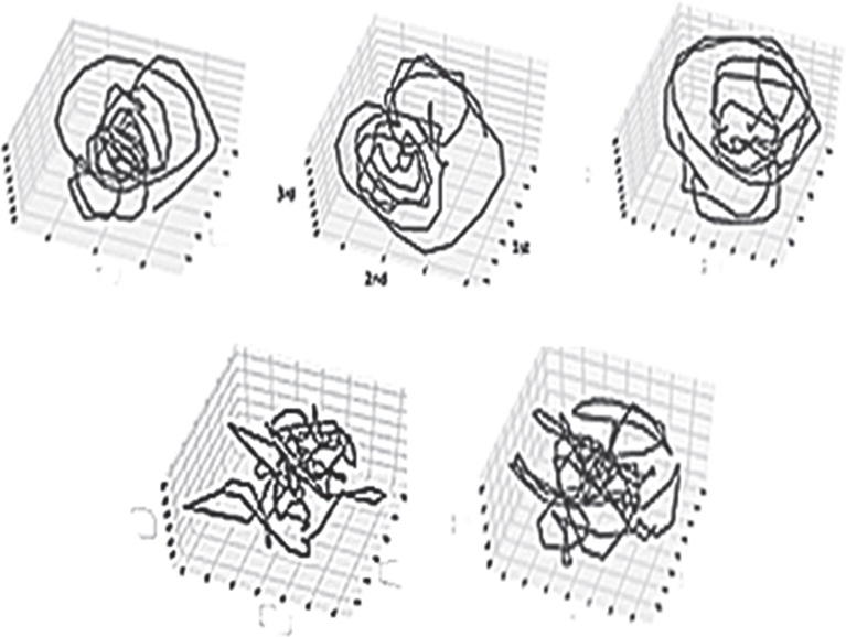
Figure 6.3 Phase-delay portraits of MEG from a central, C16, region of ssds orbits embedded in R3.
The recurrence plot [91], Figure 6.4, is an [i, j] array of dots in an n-square space in which a dot is placed at [i, j] whenever x(j) is sufficiently close to x(i) (close to be empirically defined). Recurrence plots of orbits composed of uniformly random, transitive point sets look pale and smooth, whereas orbits with intermittent “runs” of close-by values, that is, intermittency, demonstrate variously sized, denser aggregates of points. The recurrence plot of intermittent dynamics appears to “bunch up” in the recurrence plots [92]. This affords an immediate qualitative picture of the extent of the intermittency, which then can be quantified in a variety of ways including the reciprocal of the leading Lyapounov exponent, Λ, or in the form of a related computable entropy, the logarithm of the leading Lyapounov exponent, lnΛ [93] [94]. For example, given that the average Λ > 0, the longer the average relative time of laminar flow, Λ = 0, log Λ = 1, between the aperiodic bursts, the lower the value of Λ > 0.
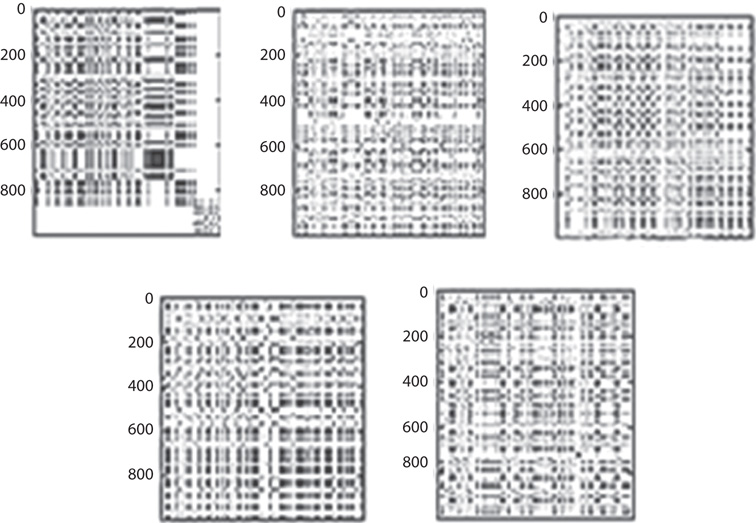
Figure 6.4 Recurrence plots corresponding to the phase space dynamics seen in Figure 6.3.
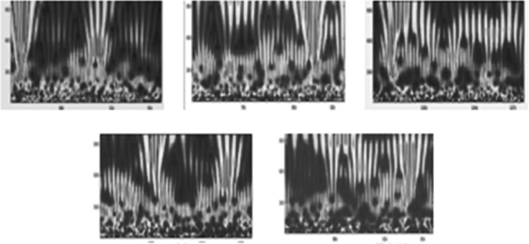
Figure 6.5 Morlet wavelet transformations of the leading autocovariance eigenfunctions of the ssds corresponding to the phase-delay portraits and recurrence plots of Figures 6.3 and 6.4.
Figure 6.5 displays the Morlet wavelet transformations of the leading autocovariance matrix eigenfunction. These results are obtained from determining the leading eigenvector of a correlation-decay-determined, lagged autocovariance matrix computed on 16.6 s of MEG (recorded at 600 Hz with 150 Hz cut-off). This leading eigenvector is then convolved with the original ssds series, leading to a new series named for their originators, Broomhead–King autocovariance eigenfunctions [95] [96]. The resulting process is analogous to what might be viewed as a leading autocovariance matrix eigenvector-weighted, nearest neighbor averaged series [97]. Morlet wavelet transformation of this autocovariance eigenfunction (Figure 6.5) demonstrates obvious intermittency in greater than three orders of magnitude of wavelengths (from 10 ms to 10 s). This results in wavelet time-frequency modes we call strudels (German for whirlpools). In dimension R3, the geometry would resemble vortices. In the context of MHD turbulence, these almost simultaneous, multiscale wavelet modes might be called turbulent eddies. They are defined generally as color-coded amplitudes originating below the bottom third of the wavelet graph and dilating past wavelet graph's upper boundary. We have speculated that these strudels, occurring in the taskless “resting” condition and occurring irregularly every 3–8 s, mirror the subjective experience of episodes of “daydreaming” [38] manifesting similar time scales [98] [99].
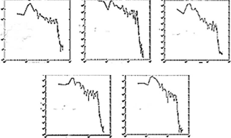
Figure 6.6 The power law scaling ssdsi characteristically ranges from 3/2 to 5/3 as seen in these log–log graphs of power (frequency) spectra. The range of exponents are consistent with both critical behavior [47] [100] and as in Figure 6.3, Figure 6.4, and Figure 6.5, turbulent intermittency. In Figure 6.6, the x axis is the log frequency and the y axis is the log power.
In Figure 6.5, notice that the intermittent and sometimes close to regular, smallest scale magnetic field activity (at the bottom of the graph) appears to seed the expansion of the strudels into larger scale, longer, mother wavelet wave lengths into the upper part and beyond of the wavelet graphs. As noted earlier, these electromagnetic dynamics are similar to those observed in studies of the “kinetic magnetic dynamo problem” in the low-resistivity domain [61] [62]. This problem as stated is “…given a flow in a conducting fluid, will a small magnetic seed amplify exponentially with time…” [29] [30, 61]. Among the possible interpretations of the strudels of Figure 6.5 are possible propagating “coherence potentials” as aggregations of critical avalanches in neocortical neural networks [47] [100] or in the context of neural network percolation theory [101]. As a smooth dynamical MHD system, these strudels are intermittent turbulent eddies [28–30] [32].
Figure 6.6 illustrates power spectra of the central, C16 ssds with similarity dimension [90] or scaling parameter, α. We minimize the mean square deviation in the middle third of the plot to estimate the log–log spectral slope yielding an f−α fractional power law, α = 1.54 ± 0.27 (n = 171). Generally, this finding is consistent with “self-similar” dynamics, manifesting a hierarchy of time scales. The observable 150 Hz acquisition cutoff serves as the upper bound on the frequency range available to examine for “scale freeness” such that the power spectral scaling approximates three orders of magnitude in range. Fractional power law, “self-similar” behavior in human MEG signals, has been reported by others as evidence of intermittent turbulent flow [90] as well as critical behavior of neuronal avalanches [47] [101]. These findings are not definitively diagnostic of either as the brain qualifies more generally as a practically infinite variable cooperative system with strong interactions and many degrees of freedom that almost always demonstrate fractional power laws [40] [72, 89]. It should also be noted that the time scale(s) of the observations, the sample length(s) being studied, and choices of relevant limit laws interact with the intrinsic dynamics such that a discriminating diagnosis using the power law scaling exponent alone is not reasonably possible.
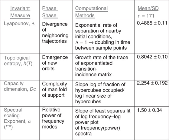
Figure 6.7 Summary of MEG ssds studies of n = 171 subjects' dynamical measures. Each value is the result of 1197 individual computations derived from the mean values of the measures obtained from seven consecutive 10 s samples from each subject recorded at 600 Hz with a 150 Hz corner frequency. In the absence of turbulence, the values would approximate, Λ ≤ 0, hT ≤ 0, DC = 3.0, and as unstructured white noise, α = 1 (log 0).
The theoretical frame of reference for the results in Figure 6.7 derive from the confluence of the Poincare–Thom's geometric-topological thinking about differential equations and Boltzmanns–Gibbs thoughts about populations, distributions of solutions to differential equations as in statistical mechanics. Behind both those points of view are last century's advances in topology, point set topology and differential topology. These gave us systematic “rules of form” such as stable and unstable fixed points, limit cycles, quasi-periodic n-tori, and chaotic attractors. It is these kinds of intuitions that underlie the current revolution in understanding of even quite subtle dynamical patterns in the data.
It is this conceptual background that has evolved into the modern “applied” ergodic theory of dynamical systems [37] [102–104]. In this context, real-valued time series can be reconstructed as phase space objects whose orbits fill up their shape (on) smooth manifolds for geometric, topological, and statistical characterization [67] [68, 105]. The Bowen shadow lemma taught us that early data points are filling up the same manifold in phase space as the later points, and the lemma states that the early points will (in an approximate way) outline the manifold(s).
Entropies (and their quasi-equivalent measures) arise as statistical invariants of those phase space objects. What is meant these days by “ergodic” is the maintenance of n, n ≤ 1, measures, μi…n in spite of (i) differing initial conditions and, often, (ii) parametric distortions of the attractor's manifold geometry short of violating its topological constraints. We study “ergodic” measures [78] on many single-orbit dynamics on these manifolds [106]. The symmetric MEG sensor difference sequences, a field property in its spatial differential form,  B(t) or in the form of our data, ssdsi, are treated as the output of dynamical systems on differentiable manifolds, here, treating the field as a manifold. Computationally, the system's dynamics can be seen as a smooth map on an n-dimensional manifold. In passing, we note that a change in topological properties such as nearness, continuity, or dimension often, if not always, is associated with the universal dynamics of phase transitions.
Figure 6.7 is a summary of the results of an n = 171 subjects study of ergodic, invariant measures [78] computed on the ssds derived from the C16 difference pairs in the MEG records of 4 min, taskless resting condition. Seven consecutive 10 s samples from each of the 171 subjects were each analyzed for the measures indicated in Figure 6.6 and then averaged to obtain that subject's values. Each individual's average was then averaged over the 171 subjects to obtain the population average for that measure. Thus, each value in Figure 6.7 is the result of 1197 individual computations of 10 s each of ssds from recordings from C16 difference pairs recorded at 600 Hz with 150 Hz cutoff. The leading Lyapounov exponent has a strongly positive average consistent with the stretch and fold dynamics of MHD turbulence; the value would be ≤0 for the nonturbulent state. Figure 6.7 shows that the lim sup of entropies, the topological entropy, hT, is also strongly positive, consistent with the value of the positive leading Lyapounov exponent and consistent with MHD turbulence.
Figure 6.7 indicates the box counting capacity dimension DC = 2.254 (fractionally less than the phase embedding space dimension of 3.0), which, in a lower dimensional, nonphysical model [30] has been attributed to the nonuniformity of the stretch and fold dynamics of MHD turbulence. The power spectral scaling exponent of approximately 3/2 (ranging up to 5/3) is consistent with the scaling exponents found in classical MHD turbulent intermittency as well as the critical behavior of neocortical neuronal network avalanches [47]. As noted, these comparisons are subject to the influence of the timescales of observations, sample lengths, and choice of limit.
From Figures 6.3 6.4, 6.5, and 6.6 and the measure table (Figure 6.7) one concludes that ssds-MEG resting record yields both qualitative graphical and quantitative measure-statistical evidence consistent with the presence of intermittent MHD turbulence in the global neocortical MEG fields. We now pursue the possibility that in addition to being representative of the human brain's global magnetic fields, measure-theoretic indications of turbulence can also be found to be discriminatively local source activity.
6.4 Localizing a Time-Varying Entropy Measure of Turbulence, Rank Vector Entropy (RVE) [35] [107], Using a Linearly Constrained Minimum Variance (LCMV) Beamformer Such as Synthetic Aperture Magnetometry (SAM) [25] [34], Yields State and Function-Related Localized Increases and Decreases in the RVE Estimate
Localization of regions of neocortical pyramidal cell networks as putative MEG sources has, until recently, been the major focus of MEG development and applications [108] [109]. The operational assumption of brain magnetic field linearity [110] supports the central role of independent static magnetic dipoles as commonly used in localization algorithms [27] [111]. Magnetic fields associated with the imposed intracellular ionic and extracellular return currents are postulated to be independent and thus directly superimposable in the determination of power. The characteristic deficiencies in matrix rank, the one to many observation-to-source, inverse MEG mapping makes more direct inverse techniques poorly approximate at best [4]. In addition, we recall that these point equivalent magnetic dipoles [51] [112, 113] are embedded in temporally and spatially fluctuating, power law distributions of turbulent magnetic fields [32] [56, 114].
A significant advance in source localization, particularly well suited for time-dependent, nonaveraged MEG signals is the volumetric mapping of estimated source activity using what has been called thesynthetic aperture magnetometer (SAM) [25] [34, 115]. It is a member of the class of minimum variance spatially filtering techniques called beamformers [116]. Generally, both the multiple dipole, LCMV beamformer [111] and the sequentially singular, four-dimensional SAM approach to localizing the time-dependent source contribution of a specific voxel involves spatial and temporal correlations or equivalent covariances [27] among the sensor array. Beamformers can be considered spatially selective filters that minimize variance (power) because of all coherent signals except for particular cerebral locations. Thus, SAM may be regarded as “spatially selective noise reduction,” where the remaining signal after minimization of all signals subject to a gain one constraint for the location being examined is an estimate of the activity at that location.
The (idealized) standard setting consists of multiple fixed, uncorrelated magnetic (linear) dipoles in a spherical, homogeneous, conducting medium with tangential sources. SAM scans in this three-dimensional, R3 space and at each position estimates the dominant dipole vector such that sources are estimated for three locations and one directional dimension in R4. By including dipolar direction in addition to location, SAM serves as a higher resolution localization technique than vector LCMV beamformers [27] [111]. Because location and volumetric complexity, rather than directionality, was the focus of this work, we have elected to use a scalar LCMV beamformer in these studies.
The assumptions of independence of the magnetic fluxes, decomposability, the finite variance of the MEG field distributions, and the associated superimpositions of linear systems all serve to support the use of the sequence of linear transformations to construct source estimates [25] [34]. However, following this localization, there is, here, a change in computational context to that of symbolic dynamics and ergodic measure theory of the nonlinear dynamics (of turbulence) [36] [84, 102] [117, 118]. Unlike most of the older techniques, the RVE does not require the difficult choices of embedding dimension and partitions of the phase space forming adjacency or transition matrices. The object of the analyses is the one-dimensional time series of the magnetic field densities as the observables [35]. The symbolic dynamic-related technique of RVE combines the topological property of order as rank [77] and the metric property of normalized probability measures over the space of available rank-ordered states [119].
The one-dimensional series of discretely sampled, MEG-recorded, magnetic flux densities, Bi…t, define a time series with t samples. Where fs defines the sample frequency and fc is the cutoff or corner frequency, lag ξ = fs/2fc is the integer intervals composing the window of W lagged samples beginning with the kth sample. Wk = [Bk, k+ξ, k+2ξ,…k+Wξ]. These measurements are then converted to their integer ranks, Rk = [Rk, k+ξ, k+2ξ,…k+Wξ] such that the number of possible rank-ordered states = W! unique symbols. The partition of states is defined by the number of discrete steps in the chosen window size; for example, a windowed ordering of W = 5 has five factorial, 5! = 120 possible integer-ordered states. As an example, the rank ordering of an MEG time series in a W = 5 window of observations: …[3.2, 4.5, 2.3, 1.1, 5.1]…would be ordered as [3, 4, 2, 1, 5] with added weight 1 to its symbol place as one of the possible orderings in the 120 place histogram, which, when normalized, becomes the probability distribution. The histogram contains the cumulative number of each rank vector state. To continue to register the local time dependence, the frequency count of the occurrence of symbols is allowed to exponentially decay with time, that is, the symbols counts are derived from a “leaky integrator.” From the histogram-derived probability distribution, the rank vector metric entropy is computed as the Shannon/Kolmogorov entropy, hrve = −Σnpnlog2pn [120] [121]. RVE remained in the turbulent regime with the median RVE ≈ 0.92 around which it decreased (coded blue) or increased (coded red) in response to perturbations by exogenous stimuli or tasks and spontaneously in the task-free, “resting” condition. Note that this value for RVE is within our standard error of the mean topological entropy, hT = 0.8042 ± 0.10, reported in the results of the 171 subject study summarized in Figure 6.7 using the entirely different algorithmic method. This serves as a quantitative validation for the new RVE entropy estimate [35].
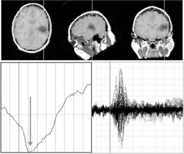
Figure 6.8 In this P300 envelope, −0.2 to +0.8 s with 100 ms intervals, the transient decrease in MEG RVE (darker grey brain areas) corresponding to the N100 localizes to the primary auditory cortex as seen in axial, sagittal, and coronal views. It accompanies an auditory evoked response to rarer tone bursts in an “odd ball” task [131], marked in time by the arrow. No characteristic changes in RVE that marked the associated P200 or P300 were observed.
The averaged MEG signal shows the prominent N100 (lower right). The averaged RVE (lower left) demonstrates a faster decrease corresponding to the N100 and a slower increase in RVE. In this study, W = 5 with 120 possible configurations of rank. The band width examined ranged from 4 to 150 Hz.
Time-locked, event-related electromagnetic responses to external, sensory, and internal, cognitive, events have often been viewed as perturbations of ongoing oscillatory (fluctuating) brain processes [122] [123]. Called EROs, event-related oscillations, they have been speculated to result from a stimulus-evoked ordering of oscillatory phase [124] [125] which can be apparent in several band widths simultaneously [126]. As in Figure 6.8, observation of the RVE decrement was found in band width of 4–150 Hz and was also observed when the generic MEG and EEG frequency bands were examined individually [35]. On the other hand, band width specificity of phase synchronization processes has also been reported to differ among brain regions and brain states [127] [128].
It is not difficult to imagine that increased coherence of phase in ongoing magnetic field turbulent oscillations could account for the apparent reduced complexity reflected in the decrement of RVE (shown as darker gray scale) as seen in Figure 6.8. Pharmacological studies have demonstrated such relationships between electromagnetic phase coherence and measures of complexity used to characterizenonlinear dynamical systems [129] [130] (Figure 6.9 and Figure 6.10).
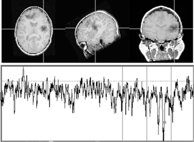
Figure 6.9 In the taskless, “resting” condition, time series of RVE (bottom) and their neuroanatomical localization (top), reveal spontaneous, multiple, intermittent, localized regions of decreased RVE (from the horizontal dotted line median ≈ 0.92). These can be seen in the axial, sagittal, and coronal views of the frontal, temporal, and parietal areas.
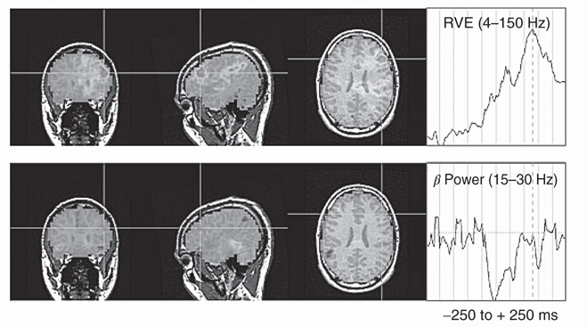
Figure 6.10 Tracking both RVE and MEG power simultaneously during 500 ms of the resting condition reveals an apparent dissociation between the time-dependent average virtual sensor's RVE and average virtual sensor's beta power (right panels) and their corresponding neocortical locations (left panels). This opens up the possibility that minimal additional energy beyond maintenance of “resting” may be required for magnetic field, neocortical entropic-informational processing. This suggests the possibility that an electromagnetic nondissipative Hamiltonian equations related to the Lorenz force may be representative of neocortical magnetic field dynamics, Section 6.3, Figure 6.1.
6.5 Potential Implications of the MHD Approach to MEG Magnetic Fields for Understanding the Mechanisms of Action and Clinical Applications of the Family of TMS (Transcranial Magnetic Stimulation) Human Brain Therapies
Experiments directed toward elucidating endogenous or exogenous field effects on brain-related dynamics until recently have been relatively rare. An early exception was the systematic studies of field effects on the behavior of large, Mauthner cells in some fish and amphibian brains [48] [132]. It was found that their associated, interleaved, parallel interneurons generated a positive extracellular current that led to a threshold increasing “down state.” The positive current field was observed to hyperpolarize the M-cell axon hillock and initial axonal segment, reducing the probability of the occurrence of action potentials. The spatial ordering of the interneurons facilitated the extracellular spread of the positive field, which inhibited or retarded M-cell depolarization. Because this effect occurred without known electrotonic gap junctions, the investigator concluded that the coupling of positive and negative fields was occurring in extracellular ionic fluid space. Similar phenomena involving the parallel arrangement of basket and pyramidal cells in the hippocampus have been reported [133] [134]. As we have noted earlier (Section 6.3 and Figure 6.1f) that from an MHD point of view, nonaxiosymmetric, near-parallel magnetic and current fields are turbulent and can exist (equivalently, identically [28]) as magnetic dynamos [28–30].
In a series of principally Russian neurophysiological studies, exogenous, weak, static, and alternating magnetic fields (sometimes DC and AC simultaneously) were shown to have intensity-dependent influences on rat behavior [135], ion flux through cellular membranes [136] [137], and ionic calcium release in brain tissue [138]. The latter has been known as the Hall effect for magnetic field influences in membranes with ion channels restrained directionally in calcium-ion-channel-containing membranes. Another, more controversial explanation of the transduction of weak magnetic field influences into biological changes involves calcium-specific 7.0 Hz electron–cyclotron resonances. This process involving the calcium ion magnetic field target for resonance was protected from aqueous dampening by its putative location in a protein hydrophobic pocket [139]. The B-field-induced changes in the electronic properties of calcium become reflected in changes in brain protein conformation via the ion's actions as an induced-fit allosteric ligand [140]. At a cellular level, exposure of pituitary corticotrope cells to calcium resonant, 7.0 Hz, 9.2 μT, weak magnetic fields have been shown to initiate neurite formation [141]. It is of particular interest that studies have emphasized the importance of the magnetic relative to the electric field in the radiation-induced efflux of calcium ions from brain tissue [142].
We postulate that the driving of endogenous brain magnetic flux fields further into the turbulent regime would be associated with increases in the brain's global field dynamical entropies (Figure 6.7). If confirmed, this effect has both pathophysiological and therapeutic significance. Over the past three decades, studies of a variety of self-excitatory biological systems [33] [40, 81] [143] have suggested that deficits in dynamical entropy and their repletion outline a scenario for a pathophysiology and treatment in dynamical disorders [144]. Augmenting the turbulence in brain magnetic field dynamics with its attendant increment in measure-theoretic entropies may be major mechanisms of action of the transcranial magnetic stimulation (TMS) therapies [145] [146]. Figure 6.11 summarizes the current and proposed theories of the action of the transcranial magnetictherapies.
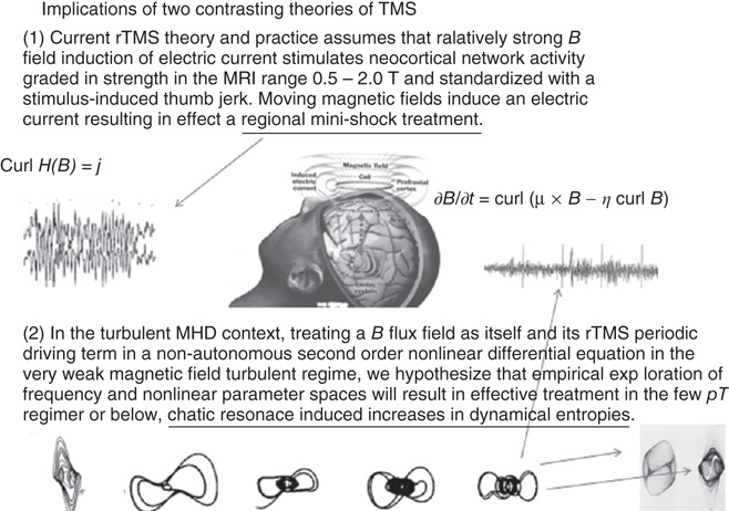
Figure 6.11 Summary of two points of view concerning the actions of the variety of transcranial magnetic stimulation therapies. (1) The strong magnetic field induction of local electrical events and (2) the weak magnetic field as a TMS-frequency-forced nonlinear dynamical system exemplifying the putative TMS entropy generation through increasing MHD turbulence. The bottom panel portrays generic quasiperiodic and chaotic attractors of the periodically driven, nonlinear van der Pol equation, which could be empirically tuned for optimal magnetic field frequency driving effect [147].
6.6 Brief Summary of Findings
- The results of the use of a set of graphical and ergodic measures on time series of central (C16) spatial derivatives of the near global neocortical magnetic field,
 = ssds, are consistent with the presence of MHD turbulence in the intermittency regime.
 - Ergodic measures on the symbolic dynamics of these magnetic flux fields are consistent with them having the capacity for quantifiable information transport.
- Beamformer localization combined with Robinson's new topological-metric entropy measure, RVE, demonstrates localized brain regions of increases and/or decreases in RVE entropy in response to auditory stimuli, cognitive tasks, and spontaneously in the “resting” condition. These localizations of entropic activity tend not to be accompanied by broad band or beta band power. This suggests that a nondissipative electromagnetic Hamiltonian treatment may be justified.
- The presence of brain magnetic-field-entropy-generating weak magnetic field turbulence, the past two decades of findings of entropy deficits in clinical brain pathophysiological dynamics, and the deficit “repair” accompanying standard therapies suggest the possibility that transcranial turbulent-entropy generation with a nonlinear dynamical system may be effective at very low field levels, pTs, in place of the large current from very much stronger magnetic field induction of local titanic activity and refractoriness.
References
- 1. Raichle, M. (2009) A paradigm shift in functional brain imaging. J. Neurosci., 29 (41), 12729–12734.
- 2. Taniguchi, M. et al. (2004) Cerebral motor control in patients with gliomas around the central sulcus studied with spatially filtered magnetoencephalography. J. Neurol. Neurosurg. Psychiatry, 75 (3), 466–471.
- 3. Anninos, P.A., Jacobson, J., Tsagas, N., and Adamopoulos, A. (1997) Spatiotemporal stationarity of epileptic focal activity evaluated by analyzing magnetoencephalographic (MEG) data and the theoretical implications. Panminerva Med., 39 (3), 189–201.
- 4. Brockhaus, A. et al. (1997) Possibilities and limitations of magnetic source imaging of methohexital-induced epileptiform patterns in temporal lobe epilepsy patients. Electroencephalogr. Clin. Neurophysiol., 102 (5), 423–436.
- 5. Llinas, R.R., Ribary, U., Jeanmonod, D., Kronberg, E., and Mitra, P.P. (1999) Thalamocortical dysrhythmia: a neurological and neuropsychiatric syndrome characterized by magnetoencephalography. Proc. Natl. Acad. Sci. U.S.A., 96 (26), 15222–15227.
- 6. Garolera, M. et al. (2007) Amygdala activation in affective priming: a magnetoencephalogram study. (Translated from eng). Neuroreport, 18 (14), 1449–1453 (in eng).
- 7. Sperling, W., Vieth, J., Martus, M., Demling, J., and Barocka, A. (1999) Spontaneous slow and fast MEG activity in male schizophrenics treated with clozapine. Psychopharmacology (Berl), 142 (4), 375–382.
- 8. Osipova, D. et al. (2003) Effects of scopolamine on MEG spectral power and coherence in elderly subjects. Clin. Neurophysiol., 114 (10), 1902–1907.
- 9. Nikulin, V.V., Nikulina, A.V., Yamashita, H., Rossi, E.M., and Kahkonen, S. (2005) Effects of alcohol on spontaneous neuronal oscillations: a combined magnetoencephalography and electroencephalography study. Prog. Neuropsychopharmacol. Biol. Psychiatry, 29 (5), 687–693.
- 10. Virji-Babul N, Cheung T, Weeks D, Herdman AT, & Cheyne D (2007) Magnetoencephalographic analysis of cortical activity in adults with and without down syndrome. J. Intellect. Disabil. Res. 51(Pt. 12):982–987.
- 11. Berendse, H.W., Verbunt, J.P., Scheltens, P., van Dijk, B.W., and Jonkman, E.J. (2000) Magnetoencephalographic analysis of cortical activity in Alzheimer's disease: a pilot study. Clin. Neurophysiol., 111 (4), 604–612.
- 12. Stoffers, D. et al. (2007) Slowing of oscillatory brain activity is a stable characteristic of Parkinson's disease without dementia. Brain, 130 (Pt 7), 1847–1860.
- 13. Canive, J.M. et al. (1996) Magnetoencephalographic assessment of spontaneous brain activity in schizophrenia. Psychopharmacol. Bull., 32 (4), 741–750.
- 14. Rutter, L. et al. (2009) Magnetoencephalographic gamma power reduction in patients with schizophrenia during resting condition. Hum. Brain Mapping, 30, 3254–3264.
- 15. Chen, Y., Ding, M., and Kelso, J.A. (2003) Task-related power and coherence changes in neuromagnetic activity during visuomotor coordination. Exp. Brain Res., 148 (1), 105–116.
- 16. Boonstra, T.W., Daffertshofer, A., Peper, C.E., and Beek, P.J. (2006) Amplitude and phase dynamics associated with acoustically paced finger tapping. Brain Res., 1109 (1), 60–69.
- 17. Cover, K.S., Stam, C.J., and van Dijk, B.W. (2004) Detection of very high correlation in the alpha band between temporal regions of the human brain using MEG. Neuroimage, 22 (4), 1432–1437.
- 18. Poza, J., Hornero, R., Abasolo, D., Fernandez, A., and Garcia, M. (2007) Extraction of spectral based measures from MEG background oscillations in Alzheimer's disease. Med. Eng. Phys., 29 (10), 1073–1083.
- 19. Liu, C., Gaetz, W., and Zhu, H. (2010) Pseudo-Differential Operators: Complex Analysis and Partial Differential Equations. Operator Theory, Advances and Applications, vol. 205, Springer, Basel, pp. 277–291.
- 20. Blank, H. et al. (1993) Dimension and entropy analyses of MEG time series from human alpha rhythm. Z. Phys. B, 91 (2), 251–256.
- 21. Fell, J., Roschke, J., Grozinger, M., Hinrichs, H., and Heinze, H. (2000) Alterations of continuous MEG measures during mental activities. (Translated from English). Neuropsychobiology, 42 (2), 99–106 (in English).
- 22. Gomez, C., Hornero, R., Abasolo, D., Fernandez, A., and Escudero, J. (2007) Analysis of MEG recordings from Alzheimer's disease patients with sample and multiscale entropies. (Translated from English). Conf. Proc. IEEE Eng. Med. Biol. Soc., 2007, 6184–6187 (in English).
- 23. Vakorin, V. (2010) Complexity analysis of source activity underlying the neuromagnetic somatosensory steady-state response. Neuroimage, 51, 83–90.
- 24. Cohen, D. (1972) Magnetoencephalography: detection of the brain's electrical activity with a superconducting magnetometer. Science, 175 (22), 664–666.
- 25. Robinson, S.E. and Vrba, J. (1999) in Recent Advances in Biomagnetism (ed. T. Yoshimoto), Tohuku University Press, Sendai, pp. 105–108.
- 26. Vrba, J. and Robinson, S.E. (1990-2011) Signal Processing in the MEG. ed. CSPort Coquitlam, Canada.
- 27. Vrba, J. and Robinson, S.E. (2000) Differences between synthetic aperture magnetometry, SAM, and linear beamformers. Biomagnetism 2000, 12th International Conference on Biomagnetism.
- 28. Radler, K.H. (1980) Mean field approach to spherical dynamo models. Astron. Nachr., 301 (H.3), 101–129.
- 29. Bayly, B. and Childress, S. (1987) Fast-dynamo action in unsteady flows and maps in three dimensions. Phys. Rev. Lett., 59, 1573–1576.
- 30. Ott, E. (1998) Chaotic flows and kinematic magnetic dynamos; a tutorial review. Phys. Plasmas, 5 (5), 1636–1646.
- 31. Alfven, H. (1942) The existence of electromagnetic-hydrodynamic waves. Nature, 150, 405–407.
- 32. Mandell, A.J., Selz, K.A., Holroyd, T., and Coppola, R. (2011) in Neuronal Variability and its Functional Significance (eds D. Glanzman and M. Ding), Oxford University Press, New York, pp. 328–390.
- 33. Mandell, A.J. (1987) Dynamical complexity and pathological order in the cardiac monitoring problem. Physica D, 27, 235–242.
- 34. Robinson, S.F. (2004) Localization of even-related activity by SAM(erf). 14th International Conference on Biomagnetism, Boston, MA, pp. 583–584.
- 35. Robinson, S.E., Mandell, A.J., and Coppola, R. (2012) Imaging complexity. BioMag 2012.
- 36. Eckmann, J.P. (1981) Roads to turbulence in dissipative dynamical systems. Rev. Mod. Phys., 53, 643–654.
- 37. Eckmann, J.P. and Ruelle, D. (1985) Ergodic theory of chaos and strange attractors. Rev. Mod. Phys., 57, 617–656.
- 38. Mandell, A.J., Selz, K.A., Aven, J., and Holroyd, T.C. (2011) in International Conference on Applications in Nonlinear Dynamics (ICAN II) (eds V. In, P. Longhini, and A. Palacios), American Institute of Physics, pp. 7–24.
- 39. Mandell, A., Selz, K., Holroyd, T., Rutter, L., and Coppola, R. (2011) in The Dynamic Brain (eds M. Ding and D. Glanzman), Oxford University Press, Oxford, pp. 296–337.
- 40. Mandell, A.J., Russo, P.V., and Knapp, S. (1982) Strange Stability in Hierarchically Coupled Neuropsychobiological Systems, Springer-Verlag, New York, pp. 270–286.
- 41. Englander, S.W., Downer, N.W., and Teitelbaum, H. (1972) Hydrogen exchange. Annu. Rev. Biochem., 41, 903–924.
- 42. Wagner, G.C., Colvin, J.T., Allen, J.P., and Stapleton, H.J. (1985) Fractal models of protein structure, dynamics and magnetic relaxation. J. Am. Chem. Soc., 107, 5589–5594.
- 43. Mandell, A.J., Stewart, K.D., Knapp, S., and Russo, P.V. (1980) Protein fluctuations and time-space asymmetries in brain [proceedings]. Psychopharmacol. Bull., 16 (4), 47–50.
- 44. Liebovitch, L.S. and Sullivan, J.M. (1987) Fractal analysis of a voltage-dependent potassium channel from cultured mouse hippocampal neurons. Biophys. J., 52 (6), 979–988.
- 45. Mandell, A.J. (1983) From intermittency to transitivity in neuropsychobiological flows. Am. J. Physiol. (Reg. Integ. Compar. Physiol.), 245 (14), R484–R494.
- 46. Paulus, M., Gass, S., and Mandell, A.J. (1989) A realistic, minimal “middle layer” for neural networks. Physica D, 40, 135–155.
- 47. Beggs, J. and Plenz, D. (2005) Neuronal avalanches are diverse and precise activity patterns that are stable for many hours in cortical slices. J. Neuosci., 24, 5216–5519.
- 48. Faber, D.S. and Korn, H. (1989) Electric field effects: their relevance in central neural networks. Physiol. Rev., 69, 821–863.
- 49. Mandell, A.J., Selz, K.A., and Shlesinger, M. (1991) in Chaos in the Brain (eds D.W. Duke and W. Pritchard), World Scientific Press, Singapore, pp. 137–155.
- 50. Frolich, F. and McCormick, D.A. (2010) Endogenous electric fields may guide neocortical network activity. Neuron, 67, 129–143.
- 51. de Munck, J., Huizenga, H., Waldorp, L., and Heethaar, R. (2002) Estimating stationary dipoles from MEG/EEG data contaminated with spatially and temporally correlated background noise. IEEE Speech Signal Process. Mag., 50 (7), 1565–1572.
- 52. de Munck, J.C., Vijn, P.C., and Lopes da Silva, F.H. (1992) A random dipole model for spontaneous brain activity. IEEE Trans. Biomed. Eng., 39 (8), 791–804.
- 53. Sato, S. and Smith, P.D. (1985) Magnetoencephalography. J. Clin. Neurophysiol., 2 (2), 173–192.
- 54. Childress, S. and Gilbert, A. (1995) Stretch, Twist, Fold: The Fast Dynamo Problem, Springer, Berlin.
- 55. Soward, A.M. (1987) Fast dynamo action in a steady flow. J. Fluid Mech., 180, 267–295.
- 56. Mandell, A.J., Selz, K.A., Aven, J., Holroyd, T., and Coppola, R. (2011) in International Conference on Applications in Nonlinear Dynamics, ICAND II (eds V. In, P. Longhini, and A. Palacios), American Institute of Physics Conference Proceedings, Lake Louise, pp. 7–24.
- 57. Heisenberg, W. (1948) On the theory of statistical and isotropic turbulence. Proc. Roy. Soc. (London), 195, 402–406.
- 58. Chandrasekhar, S. (1961) Hydrodynamic and Hydromagnetic Stability, Oxford University Press, Oxford.
- 59. Nunez, M.J. and Srinivasan, R. (2006) Electric Fields of the Brain; The Neurophysics of the EEG, Oxford University Press, Oxford.
- 60. Moffatt, H.K. (1989) Stretch, twist and fold. Nature, 341, 285–286.
- 61. Finn, J.M. and Ott, E. (1988) Chaotic flows and magnetic dynanamos. Phys. Rev. Lett., 60, 760–763.
- 62. Ott, E., Du, Y., Sreenivasan, K.R., Juneja, A., and Suri, A.K. (1992) Sing-singular measures: fast magnetic dynamos and high Reynolds-number fluid turbulence. Phys. Rev. Lett., 69, 2654–2657.
- 63. Maruoka, H., Kubota, K., Kurokawa, R., Tsuruno, S., and Hosoya, T. (2011) Periodic organization of major subtype of pyramidal cell neurons in neocortical layer V. J. Neurosci., 31, 18522–16542.
- 64. Gurnett, D. and Bhattacharjee, A. (2005) Introduction to Plasma Physics: With Space and Laboratory Applications, Cambridge University Press, Cambridge.
- 65. Griffiths, D.J. (1999) Introduction to Electrodynamics, Prentice Hall, Saddle River, NJ.
- 66. Aven, J.L., Mandell, A.J., Holroyd, T., and Coppola, R. (2011) Complexity of the taskless mind at different time scales.an emperically weighted approach to decomposition and measurement. AIP Conf. Proc., 1339, 275–281.
- 67. Smale, S. (1967) Differentiable dynamical systems. Bull. AMS, 73, 747–817.
- 68. Bowen, R. (1978) On Axiom A Diffeomorphisms, A.M.S. Publications.
- 69. Mandell, A.J. and Selz, K.A. (1997) Entropy conservation as topological entropy = leading Lyapounov exponent times the capacity dimension. Chaos, 7, 67–81.
- 70. Galaburda, A.M., LeMay, M., Kemper, T.L., and Geschwind, N. (1978) Right-left asymmetrics in the brain. Science, 199 (4331), 852–856.
- 71. Cowling, T.G. (1933) Axiosymmetry in Static Magnetic Fields, MNRAS 94, Monthly Notice of the Royal Astronomical Society.
- 72. Novikov, E., Novikov, A., Shannahoff-Khalsa, D., Schwartz, B., and Wright, J. (1997) Scale-similar activity in the brain. Phys. Rev. E, 56, R2387–R2389.
- 73. DeFelice, L.J. (1977) Fluctuation analysis in neurobiology. Int. Rev. Neurobiol., 20, 169–208.
- 74. Conti, F., Neumcke, B., Nonner, W., and Stampfli, R. (1980) Conductance fluctuations from the inactivation process of sodium channels in myelinated nerve fibres. (Translated from English). J. Physiol., 308, 217–239 (in English).
- 75. Sigworth, F.J. (1981) Interpreting power spectra from nonstationary membrane current fluctuations. (Translated from English). Biophys. J., 35 (2), 289–300 (in English).
- 76. Ornstein, D.S. (1974) Ergodic Theory, Randomness and Dynamical Systems, Yale University Press, New Haven, CT.
- 77. Adler, R.L. and Weiss, B. (1967) Entropy, a complete metric invariant for automorphisms of the torus. Proc. Natl. Acad. Sci. U.S.A., 57, 1573–1576.
- 78. Cornfield, I., Fomin, V., and Sinai, Y. (1982) Ergodic Theory, Springer-Verlag, Berlin.
- 79. Mandell, A., Selz, K.A., and Shlesinger, M.F. (1991) in Chaos in the Brain (eds D.W. Duke and W.S. Pritchard), World Scientific Press, Hong Kong, pp. 174–190.
- 80. Mandell, A.J. and Selz, K.A. (1995) Nonlinear dynamical patterns as personality theory for neurobiology and psychiatry. Psychiatry, 58 (4), 371–390.
- 81. Mandell, A.J. and Shlesinger, M.F. (1990) Lost Choices; Parallelism and Topological Entropy Decrements in Neurobiological Aging, American Association for the Advancement of Science, Washington, DC, pp. 10–22.
- 82. Smotherman, W.P., Selz, K.A., and Mandell, A.J. (1996) Dynamical entropy is conserved during cocaine-induced changes in fetal rat motor patterns. Psychoneuroendocrinology, 21 (2), 173–187.
- 83. Bowen, R. and Ruelle, D. (1975) The ergodic theory of Axiom A flows. Invent Math., 29, 181–202.
- 84. Frisch, U. (1995) Turbulence: The Legacy of A.N. Kolmogorov, Cambridge University Press, Cambridge.
- 85. Manneville, P. and Pomeau, Y. (1980) Different ways to turbulence in dissipative dynamical systems. Physica D, 1, 219–232.
- 86. Berge, P., Pomeau, Y., and Vidal, C. (1984) Order and Chaos, Chapter IX. Intermittency , John Wiley & Sons, Inc./Hermann, New York/Paris, pp. 223–247.
- 87. Segundo, J.P., Sugihara, G., Dixon, P., Stiber, M., and Bersier, L.F. (1998) The spike trains of inhibited pacemaker neurons seen through the magnifying glass of nonlinear analyses. Neuroscience, 87 (4), 741–766.
- 88. Mandell, A.J. and Selz, K.A. (1993) Brain stem neuronal noise and neocortical “resonance”. J. Stat. Phys., 70, 355–373.
- 89. Mandell, A. and Selz, K.A. (1991) in Self-Organization, Emerging Properties and Learning (ed. A. Babloyantz), Plenum Press, New York, pp. 255–266.
- 90. Novikov, A. (1990) The effects of intermittency on statistical characteristics of turbulence and scale similarity of breakdown coefficients. Phys. Fluids, 2, 614–620.
- 91. Eckmann, J.P., Kamhorst, S., and Ruelle, D. (1987) Recurrence plots of dynamical systems. Europhys. Lett., 4, 973–977.
- 92. Mandell, A.J. and Selz, K.A. (1997) Entropy conservation as Topological entropy = Lyapounov*Capacity Dimension in neurobiological dynamical systems. J. Chaos, 7, 67–91.
- 93. Pesin, Y. (1977) Characteristic Lyapounov exponents and smooth ergodic theory. Russ Math. Surv., 32, 55–114.
- 94. Paulus, M.P., Geyer, M.A., Gold, L.H., and Mandell, A.J. (1990) Application of entropy measures derived from the ergodic theory of dynamical systems to rat locomotor behavior. Proc. Natl. Acad. Sci. U.S.A., 87 (2), 723–727.
- 95. Broomhead, D.S. and King, G.P. (1986) Extracting qualitative dynamics from experimental data. Physica D, 20, 217–236.
- 96. Broomhead, D.S., Jones, R., and King, G.P. (1987) Addenda and correction. J. Phys. A, 20, L563–L569.
- 97. Mandell, A.J., Selz, K.A., Owens, M.J., and Shlesinger, M.F. (2003) in Unsolved Problems of Noise and Fluctuations (ed. S.M. Bezrukov), American Institute of Physics Press, Melville, New York, pp. 553–559.
- 98. Singer, J.L. (1966) Daydreaming: A Introduction to the Experimental Study of Inner Experience, Random House, New York.
- 99. Antrobus, J.S., Singer, J.L., and Greenberg, S. (1966) Studies in the stream of consciousness:experimental enhancement and suppression of spontaneous cognitive processes. Percept. Mot. Skills, 23, 399–417.
- 100. Petermannan, T. et al. (2009) Spontaneous cortical activity in awake monkeys composed of neuronal avalanches. Proc. Natl. Acad. Sci. U.S.A., 106, 15921–15926.
- 101. Stauffer, D. and Aharony, A. (1994) Introduction to Percolation Theory, 2nd edn, CRC Press, Florence, KY.
- 102. Kolmogorov, A.N. (1957) General theory of dynamical systems and classical mechanics. Proc. Internat. Cong. Math., 1, 315–333.
- 103. Arnold, V.I. and Avez, A. (1968) Ergodic Problems of Classical Mechanics, Addison-Wesley, Reading.
- 104. Arnold, V.I. (1983) Geometrical Methods in the Theory of Ordinary Differential Equations, Springer-Verlag, New York.
- 105. Sinai, Y. (1970) Dynamical systems with countably-multiple Lebesgue spectrum. Trans. AMS, 68, 34–88.
- 106. Weiss, B. (1995) Single Orbit Dynamics (Reg. Conf. # 95), American Mathematical Society, Providence, RI.
- 107. Robinson, S.E., Mandell, A.J., and Coppola, R. (2012) Imaging complexity. BioMag 2012.
- 108. Wikswo, J. (1989) in Advances in Biomagnetism (eds S.J. Williamson, M. Hoke, G. Stroink, and M. Kotani), Plenum, New York, pp. 1–18.
- 109. Williamson, S.J., Lu, Z.L., Karron, D., and Kaufman, L. (1991) Advantages and limitations of magnetic source imaging. Brain Topogr., 4 (2), 169–180.
- 110. Babiloni, F. et al. (2001) Linear inverse source estimate of combined EEG and MEG data related to voluntary movements. (Translated from English). Hum. Brain Mapp., 14 (4), 197–209, (in English).
- 111. Vrba, J. and Robinson, S.E. (2000) IEEE Proceeding of the 34th Asimilar Conference on Signals, Systems and Computers, Omnipress, Madison, WI, pp. 313–317.
- 112. Scherg, M. and von Cramon, D. (1985) A new interpretation of the generators of BAEP waves I-V: Results of a spatio-temporal dipole model. EEG Clin. Neurophys., 62, 290–299.
- 113. Vrba, J. and Robinson, S.E. (2002) SQUID sensor array configurations for magnetoencephalography applications. Supercond. Sci. Technol., 15, R51–R89.
- 114. Mandell, A. and Selz, K.A. (1992) in Proceedings of the First Experimental Conference on Chaos (eds S. Vohra, M.L. Spano, M. Shlesinger, L. Pecora, and W. Ditto), World Scientific Press, Singapore, pp. 175–191.
- 115. van Veen, B.D. and Buckley, K.M. (1988) Beamforming: a versatile approach to spatial filtering. IEEE Accoust. Speach Signal Process. Mag., 5, 4–24.
- 116. Vrba, J. and Robinson, S. (2001) Signal processing in magnetoencephalography. Methods(Duluth), 25, 249–271.
- 117. Kolmogorov, A.N. (1941) The local structure of turbulence in viscous incompressible fluid at very large Reynold's numbers. Dokl. Akad. Nauk SSSR, 30, 301–305.
- 118. Morse, M. and Hedlund, G.A. (1938) Symbolic dynamics. Am. J. Math., 60, 815–866.
- 119. Adler, R.L., Goodwyn, L.W., and Weiss, B. (1977) Equivalence of Markoff shifts. Isr. J. Math., 27, 49–63.
- 120. Shannon, C.E. (1948) A mathematical theory of communication. Bell. Syst. Tech. J., 27, 379–423.
- 121. Kolmogorov, A.N. (1958) A new metric invariant of transitive dynamical systems and automorphisms in Lebesgue spaces. Dokl. Acad. Nauk. SSSR, 119, 861–882.
- 122. Basar, E., Flohr, H., Haken, H., and Mandell, A.J. (1983) Synergetics Brain, Springer-Verlag, Berlin.
- 123. Basar, E. (1980) EEG-Brain Dynamics; Relations Between EEG and Brain Evoked Potentials, Elsevier, Amsterdam.
- 124. Basar, E., Basar-Eroglu, C., Karakas, S., and Schurmann, M. (2000) Brain oscillations in perception and memory. J. Psychophysiol., 35, 95–124.
- 125. Roach, B. and Mathalon, D. (2008) Event-related time-frequency analysis: an overview of measures and an analysis of early gamma band phase locking in schizophrenia. Schizophr. Bull., 34, 907–926.
- 126. Makeig, S. et al. (2002) Dynamic brain sources of visual evoked responses. Science, 295, 690–694.
- 127. Kopell, N., Ermentrout, G., Whittington, M., and Traub, R.D. (2000) Gamma rhythms and beta rhythms have different synchronization properties. Proc. Natl. Acad. Sci. U.S.A., 97, 1867–1872.
- 128. Ehlers, C., Wills, D.N., and Havstad, J. (2012) Ethanol reduces the phase locking of neural activity inn human and rodent brain. Brain Res., 1450, 67–79.
- 129. Ehlers, C. (1992) The new physics of chaos: can it help us to understand the effects of alcohol. Alcohol Health Res. World, 16, 267–272.
- 130. Ehlers, C., Havstad, J., Pritchard, D., and Theiler, J. (1998) Low doses of ethanol reduce evidence for nonlinear structure in brain activity. J. Neurosci., 18, 7474–7486.
- 131. Donchin E, Ritter W, & McCallum C (1978) in Brain-Event Related Potentials in Man, eds Callaway E, Tueting P, & Koslow S Academic Press, pp. 349-411.
- 132. Faber, D.S. and Korn, H. (1973) A neuronal inhibition mediated electrically. Science, 179, 577–578.
- 133. Pare, D., Shink, E., Gaudreau, H., and Destexhe, A. (1998) Impact of spontaneous synaptic activity on the resting properties of cat neocortical pyramidal neurons in vivo. J. Neurophysiol., 79, 1450–1460.
- 134. Palay, S.L. and Chan-Palay, V. (1974) Cerebellar Cortex, Cytology and Organization, Springer-Verlag, Berlin.
- 135. Liboff, A.R., Thomas, J.R., and Schrot, J. (1988) Intensity threshold for 60 Hz magnetically induced behavioral changes in rats. Bioelectromagnetics, 10, 1–3.
- 136. McLeod, B. and Liboff, A.R. (1986) Dynamic characteristics of membrane ions in multifield configurations of low-frequency electromagnetic radiation. Bioelectromagnetics, 7, 177–189.
- 137. Liboff, A. and McLeod, B.R. (1988) Kinetics of channelized membrane ions in magnetic fields. Bioelectromagnetics, 9, 39–51.
- 138. Black Man, C., Benane, S.G., Elliott, D.J., House, D.E., and Pollock, M.M. (1988) Influence of electromagnetic fields on the efflux of calcium ions from brain tissue. Bioelectromagnetics, 9, 215–227.
- 139. Lednev, V.V. (1991) Possible mechanism for the influence of weak magnetic fields on biological systems. Bioelectromagnetics, 12, 71–75.
- 140. Knapp, S., Mandell, A.J., and Bullard, W.P. (1975) Calcium activation of brain tryptophan hydroxylase. Life Sci., 16 (10), 1583–1593.
- 141. Ledda, F., De Carlo, F., Grimaldi, S., and Lisi, A. (2010) Calcium ion cyclotron resonance, ICR, at 7.0 Hz, 9.2 micro-Tesla magnetic field exposure initiates differentiation of pituitary corticotrope-derived AtT20 D16V cells. Electromagn. Biol. Med., 29, 63–71.
- 142. Black Man, C., Benane, S.G., Rabinowitz, J., House, D.E., and Joines, W. (1985) A role for the magnetic field in the radiation-induced efflux of calcium ions from brain tissue in vitro. Bioelectromagnetics, 6, 327–337.
- 143. Hausdorff, J.M., Herman, T., Baltadjieva, R., Gurevich, T., and Giladi, N. (2003) Balance and gait in older adults with systemic hypertension. Am. J. Cardiol., 91 (5), 643–645.
- 144. Mackey, M. and Glass, L. (1977) Oscillations and chaos in physiological control systems. Science, 197, 287–289.
- 145. George, M. (2003) Stimulating the brain: the emerging new science of electrical brain stimulation. Sci. Am., 289, 66–73.
- 146. George, M.S. and Belmaker, R.H. (2007) Transcranial Magnetic Stimulation in Clinical Psychiatry, American Psychiatric Publishing, Washington, DC.
- 147. Mandell, A.J., Russo, P.V., and Blomgren, B.W. (1987) Geometric universality in brain allosteric protein dynamics; complex hydrophobic transformation predicts mutual recognition by polypeptides and proteins. Ann. N.Y. Acad. Sci., 504, 88–117.