7
Thermodynamic Model of Criticality in the Cortex Based on EEG/ECoG Data

Robert Kozma, Marko Puljic and Walter J. Freeman

Prologue …Thus logics and mathematics in the central nervous system, when viewed as languages, must structurally be essentially different from those languages to which our common experience refers. … whatever the system is, it cannot fail to differ considerably from what we consciously and explicitly considered as mathematics, von Neumann [1].

7.1 Introduction

Von Neumann emphasized the need for new mathematical disciplines in order to understand and interpret the language of the brain [1]. He has indicated the potential directions of such new mathematics through his work on self-reproducing cellular automata and finite mathematics. Owing to his early death in 1957, he was unable to participate in the development of relevant new theories, including morphogenesis pioneered by Turing [2] and summarized by Katchalsky [3]. Prigogine [4] developed this approach by modeling the emergence of structure in open chemical systems operating far from thermodynamic equilibrium. He called the patterns dissipative structures, because they emerged by the interactions of particles feeding on energy with local reduction in entropy. Haken [5] developed the field of synergetics, which is the study in lasers of pattern formation by particles, whose interactions create order parameters by which the particles govern themselves in circular causality.

Principles of self-organization and metastability have been introduced to model cognition and brain dynamics [6–8]. Recently, the concept of self-organized criticality (SOC) has captured the attention of neuroscientists [9]. There is ample empirical evidence of the cortex conforming to the self-stabilized, scale-free dynamics of the sandpile during the existence of quasi-stable states [10–12]. However, the model cannot produce the emergence of orderly patterns within a domain of criticality [13, 14]. In [15] SOC is described as “pseudocritical” and it is suggested that self-organization be complemented with more elaborate, adaptive approaches.

Extending on previous studies, we propose to treat cortices as dissipative thermodynamic systems that by homeostasis hold themselves near a critical level of activity far from equilibrium but steady state, a pseudoequilibrium. We utilize Freeman's neuroscience insights manifested in the hierarchical brain model: the K (Katchalsky)-sets [3, 16]. Originally, K-sets have been described mathematically using ordinary differential equations (ODEs) with distributed parameters and with stochastic differential equations (SDEs) using additive and multiplicative noise [17, 18]. This approach has produced significant results, but certain shortcomings have been pointed out as well [19–21]. Calculating stable solutions for large matrices of nonlinear ODE and SDE closely corresponding to chaotic electrocorticography (ECoG) activity are prohibitively difficult and time consuming on both digital and analog platforms [22]. In addition, there are unsolved theoretical issues in constructing solid mathematics with which to bridge the difference across spatial and temporal scales between microscopic properties of single neurons and macroscopic properties of vast populations of neurons [23, 24].

In the past decade, the neuropercolation approach has proved to be an efficient tool to address these shortcomings by implementing K-sets using concepts of discrete mathematics and random graph theory (RGT) [25]. Neuropercolation is a thermodynamics-based random cellular neural network model, which is closely related to cellular automata (CA), the field pioneered by von Neumann, who anticipated the significance of CA in the context of brain-like computing [26]. This study is based on applying neuropercolation to systematically implement Freeman's principles of neurodynamics. Brain dynamics is viewed as a sequence of intermittent phase transitions in an open system, with synchronization–desynchronization effects demonstrating symmetry breaking demarcated by spatiotemporal singularities [27–30].

This work starts with the description of the basic building blocks of neurodynamics. Next, we develop a hierarchy on neuropercolation models with increasing complexity in structure and dynamics. Finally, we employ neuropercolation to describe critical behavior of the brain and to interpret experimentally observed ECoG/EEG (electroencephalography) dynamics manifesting learning and higher cognitive functions. We conclude that criticality is a key aspect of the operation of the brain and it is a basic attribute of intelligence in animals and in man-made devices.

7.2 Principles of Hierarchical Brain Models

7.2.1 Freeman K-Models: Structure and Functions

We propose a hierarchical approach to spatiotemporal neurodynamics, based on K-sets. Low-level K-sets were introduced by Freeman in the 1970s, named in honor of Aharon Kachalsky, an early pioneer of neural dynamics [16]. K-sets are multiscale models, describing the increasing complexity of structure and dynamical behaviors. K-sets are mesoscopic models, and represent an intermediate level between microscopic neurons and macroscopic brain structures. The basic K0 set describes the dynamics of a cortical microcolumn with about neurons. K-sets are topological specifications of the hierarchy of connectivity in neuron populations. When first introduced, K-sets were modeled using a system of nonlinear ODEs; see [16, 21]. K-dynamics predict the oscillatory waveforms that are generated by neural populations. K-sets describe the spatial patterns of phase and amplitude of the oscillations. They model observable fields of neural activity comprising EEG, local field potential (LFP), and magnetoencephalography (MEG). K-sets form a hierarchy for cell assemblies with the following components[31]:

• K0 sets represent noninteractive collections of neurons with globally common inputs and outputs: excitatory in K0e sets and inhibitory in K0isets. The K0 set is the basic module for K-sets.
• KI sets are made of a pair of interacting K0 sets, both either excitatory or inhibitory in positive feedback. The interaction of K0e sets gives excitatory bias; that of K0i sets sharpens input signals.
• KII sets are made of a KIe set interacting with a KIi set in negative feedback, giving oscillations in the gamma and high beta range (20–80 Hz). Examples include the olfactory bulb and the prepyriform cortex.
• KIII sets are made up of multiple interacting KII sets. Examples include the olfactory system and the hippocampal system. These systems can learn representations and do match–mismatch processing exponentially fast by exploiting chaos.
• KIV sets made up of interacting KIII sets are used to model multisensory fusion and navigation by the limbic system.
• KV sets are proposed to model the scale-free dynamics of neocortex operating on and above KIV sets in mammalian cognition.

K-sets are complex dynamical systems modeling the classification in various cortical areas, having typically hundreds or thousands of degrees of freedom. KIII sets have been applied to solve various classification and pattern recognition problems [21, 32, 33]. In early applications, KIII sets exhibited extreme sensitivity to model parameters, which prevented their broad use in practice [32]. In the past decade, systematic analysis has identified regions of robust performance and stability properties of K-sets have been derived [34, 35]. Today, K-sets are used in a wide range of applications, including detection of chemicals [36], classification [32, 37], time series prediction [38], and robot navigation [39, 40].

7.2.2 Basic Building Blocks of Neurodynamics

The hierarchical K-model-based approach is summarized in the 10 Building Blocks of Neurodynamics; see [16, 23, 24]:

1. Nonzero point attractor generated by a state transition of an excitatory population starting from a point attractor with zero activity. This is the function of the KI set.
2. Emergence of damped oscillation through negative feedback between excitatory and inhibitory neural populations. This is the feature that controls the beta–gamma carrier frequency range and it is achieved by KII having low feedback gain.
3. State transition from a point attractor to a limit cycle attractor that regulates steady-state oscillation of a mixed E-I KII cortical population. It is achieved by KII with sufficiently high feedback gain.
4. The genesis of broad-spectral, aperiodic/chaotic oscillations as background activity by combined negative and positive feedback among several KII populations; achieved by coupling KII oscillators with incommensurate frequencies.
5. The distributed wave of chaotic dendritic activity that carries a spatial pattern of amplitude modulation (AM) in KIII.
6. The increase in nonlinear feedback gain that is driven by input to a mixed population, which results in the destabilization of the background activity and leads to emergence of an AM pattern in KIII as the first step in perception.
7. The embodiment of meaning in AM patterns of neural activity shaped by synaptic interactions that have been modified through learning in KIII layers.
8. Attenuation of microscopic sensory-driven noise and enhancement of macroscopic AM patterns carrying meaning by divergent–convergent cortical projections in KIV.
9. Gestalt formation and preafference in KIV through the convergence of external and internal sensory signals, leading to the activation of the attractor landscapes and from there to intentional action.
10. Global integration of frames at the theta rates through neocortical phase transitions representing high-level cognitive activity in the KV model.

Principles 1 through 7 describe the steps toward basic sensory processing, including pattern recognition, classification, and prediction, which is the function of KIII models. Principles 8 and 9 reflect the generation of basic intentionality using KIV sets. Principle 10 expresses the route to high-level intentionality and ultimately consciousness. The greatest challenge in modeling cortical dynamics is posed by the requirement to meet two seemingly irreconcilable requirements. One is to model the specificity of neural action even to the level that a single neuron can be shown to have the possibility of capturing brain output. The other is to model the generality by which neural activity is synchronized and coordinated throughout the brain during intentional behavior. Various sensory cortices exhibit great similarity in their temporal dynamics, including the presence of spontaneous background activity, power-law distribution of spatial and temporal power spectral densities, repeated formation of AM spatial patterns with carrier frequencies in the beta and gamma ranges, and frame recurrence rates in the theta range.

Models based on ODE and SDE have been used successfully to describe the mesoscopic dynamics of cortical populations for autonomous robotics [40, 41]. However, such approaches suffered from inherent shortcomings. They falter in attempts to model the entire temporal and spatial range including the transitions between levels, which appear to take place very near to criticality. Neuropercolation and RGT offer a new approach to describe critical behavior and related phase transitions in the brain. It is shown that criticality in the neuropil is characterized by a critical region instead of a singular critical point, and the trajectory of the brain as a dynamical systems crosses the critical region from a less organized (gaseous) phase to more organized (liquid) phase during input-induced destabilization and vice versa [42–44]. Neuropercolation is able to simulate these important results from mesoscopic ECoG/EEG recording across large spacial and temporal scales, as is introduced in this chapter.

7.2.3 Motivation of Neuropercolation Approach to Neurodynamics

We utilize the powerful tools of RGT developed over the past 50 years [45–47] to establish rigorous models of brain networks. Our model incorporates CA and percolation theory in random graphs that are structured in accordance with cortical architectures. We use the hierarchy of interactive populations in networks as developed in Freeman K-models [16], but replace differential equations with probability distributions from the observed random graph that evolve in time. The corresponding mathematical object is called neuropercolation [25]. Neuropercolation theory provides a suitable mathematical approach to describe phase transitions and critical phenomena in large-scale networks. It has potential advantage compared to ODEs and partial differential equations (PDEs) when modeling spatiotemporal transitions in the cortex, as differential equations assume some degree of smoothness in the described phenomena, which may not be very suitable to model the observed sudden changes in neurodynamics. The neural percolation model is a natural mathematical domain for modeling collective properties of brain networks, especially near critical states, when the behavior of the system changes abruptly with the variation of some control parameters.

Neuropercolation considers populations of cortical neurons that sustain their metastable state by mutual excitation, and its stability is guaranteed by the neural refractory periods. Nuclear physicists have used the concept of criticality to denote the threshold for ignition of a sustained nuclear chain reaction, that is, fission. The critical state of nuclear chain reaction is achieved by a delicate balance between the material composition of the reactor and its geometrical properties. The criticality condition is expressed as the identity of geometrical curvature (buckling) and material curvature. Chain reactions in nuclear processes are designed to satisfy strong linear operational regime conditions, in order to assure stability of the underlying chain reaction. That usage fails to include the self-regulatory processes in systems with nonlinear homeostatic feedback that characterize cerebral cortices.

A key question is how the cortex transits between gas-like randomness and liquid-like order near the critical state. We have developed thermodynamic models of the cortex [43, 44], which postulate two phases of neural activity: vapor-like and liquid-like. In the vapor-like phase, the neurons are uncoupled and maximally individuated, which is the optimal condition for processing microscopic sensory information at low density. In the liquid-like phase, the neurons are strongly coupled and thereby locked into briefly stable macroscopic activity patterns at high density, such that every neuron transmits to and receives from all other neurons by virtue of small-world effects [48, 49]. Local 1/f fluctuations have the form of phase modulation (PM) patterns that resemble droplets in vapor. Large-scale, spatially coherent AM patterns emerge from and dissolve into this random background activity but only on receiving conditioned stimulus (CS). They do so by spontaneous symmetry breaking [42] in a phase transition that resembles condensation of a raindrop, in that it requires a large distribution of components, a source of transition energy, a singularity in the dynamics, and a connectivity that can sustain interaction over relatively immense correlation distances. We conclude that the background activity at the pseudoequilibrium state conforms to SOC, that the fractal distribution of phase patterns corresponds to that of avalanches, that the formation of a perception from sensory input is by a phase transition from a gas-like, disorganized, low-density phase to a liquid-like high-density phase [43].

7.3 Mathematical Formulation of Neuropercolation

7.3.1 Random Cellular Automata on a Lattice

In large networks, such as the cortex, organized dynamics emerges from the noisy and chaotic behavior of a large number of microscopic components. Such systems can be modeled as graphs, in which neurons become vertices. The activity of every vertex evolves in time depending on its own state, the states of its neighbors, and possibly some random influence. This leads us to the general formulation of random CA. In a basic two-state cellular automaton, the state of any lattice point is either active or inactive. The lattice is initialized with some (deterministic or random) configuration. The states of the lattice points are updated (usually synchronously) on the basis of some (deterministic or probabilistic) rule that depends on the activations of their neighborhood. For related general concepts, see CA such as Conway's Game of Life, cellular neural network, as well as thermodynamic systems like the Ising model [50–53]. Neuropercolation models develop neurobiologically motivated generalizations of CA models and incorporate the following major conditions:

• Interaction with noise: The dynamics of the interacting neural populations is inherently nondeterministic due to dendritic noise and other random effects in the nervous tissue and external noise acting on the population. Randomness plays a crucial role in neuropercolation models and there is an intimate relationship between noise and the system dynamics, because of the excitable nature of the neuropil.
• Long axon effects (rewiring): Neural populations stem ontogenetically in embryos from aggregates of neurons that grow axons and dendrites and form synaptic connections of steadily increasing density. At some threshold, the density allows neurons to transmit more pulses than they receive, so that an aggregate undergoes a state transition from a zero point attractor to a nonzero point attractor, thereby becoming a population. In neural populations, most of the connections are short, but there are a relatively few long-range connections mediated by long axons. The effects of long-range axons are similar to small-world phenomena [48] and it is part of the neuropercolation model.
• Inhibition: An important property of neural tissue is that it contains two basic types of interactions: excitatory and inhibitory ones. Increased activity of excitatory populations positively influence (excite) their neighbors, while highly active inhibitory neurons negatively influence(inhibit) the neurons they interact with. Inhibition is inherent in cortical tissues and it controls stability and metastability observed in brain behaviors [7, 35]. Inhibitory effects are part of neuropercolation models.

7.3.2 Update Rules

A vertex of a graph is in one of two states, , and influenced via the edges by neighbors. An edge from to , , either excites and inhibits. Excitatory edges project the states of neighbors and inhibitory edges project the opposite states of neighbors, 0 if the neighbor's state is 1, and 1 if it is 0. The state of the vertex, influenced by edges, is determined by the majority rule; the more neighbors are active, the higher the chance for the vertex to be active; and the more neighbors are inactive, the higher the chance for the vertex to be inactive. At time is randomly set to or . Then, for , a majority rule is applied simultaneously over all vertices. A vertex is influenced by a state of its neighbor , whenever a random variable is less than the influencing excitatory edge strength, , else the vertex is influenced by an opposite state of neighbor . If the edge is inhibitory, the vertex sends 0 when , and 1 when . Then, a vertex gets a state of the most common influence, if there is one such; otherwise, a vertex state is randomly set to 0 or 1, Figure 7.1a.

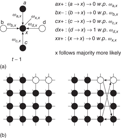
Figure 7.1 Illustration of update rules in 2D lattice. (a) An example of how majority function works. edge inhibits with strength , so it sends 0 when . Given the scenario, is 0 most likely. (b): Example of 2D torus of order . First row/column is connected with last row/column. Each vertex has a self-influence. Right: 2D torus after the basic random rewiring strategy. Two out of 80 () edges are rewired or 2.5%.

Formula for the majority rule:

7.1

7.3.3 Two-Dimensional Lattice with Rewiring

Lattice-like graphs are built by randomly reconnecting some edges in the graphs set on a regular two-dimensional grid in and folded into tori. In the applied basic random rewiring strategy, directed edges from vertices are plugged out from a graph randomly. At that point, the graph has vertices lacking an incoming edge and vertices lacking an outgoing edge. To preserve the vertex degrees of the original graph, the set of plugged-out edges is returned to the vertices with the missing edges in random order. An edge is pointed to the vertex missing the incoming edge and is projected from the vertex missing the outgoing edge, Figure 7.1b. Such a two-dimensional graph models a KI set with a homogeneous population of excitatory and inhibitory neurons.

It will be useful to reformulate the basic subgraph on a regular grid, as shown in Figure 7.2. We list all vertices along a circle and connect the corresponding vertices to obtain the circular representation on Figure 7.2b. This circle is unfolded into a linear band by cutting it up at one location, as shown in Figure 7.2c. Such a representation is very convenient for the design of the rewiring algorithm. Note that this circular representation is not completely identical to the original lattice, owing to the different edges when folding the lattice into a torus. We have conducted experiments to compare the two representations and obtained that the difference is minor and does not affect the basic conclusions. An important advantage of this band representation that it can be generalized to higher dimensions by simply adding suitable new edges between the vertices. For example, in 2D we have four direct neighbors and thus four connecting edges; in 3D, we have six connecting edges, and so on. Generalization to higher dimensions is not used in this work as the 2D model is a reasonable approximation of the layered cortex.

Figure 7.2 (a) Example of a labeled torus in two-dimension. (b) Conversion of the2D lattice approximately into a 2D torus where vertices are set in a circle.(c) 2D torus cut an unfolded into a linear band. (d) Illustration of theneighborhoods in higher dimensions.

7.3.4 Double-Layered Lattice

We construct a double-layered graph by connecting two lattices (see Figure 7.3(a)). The top layer is excitatory, while the bottom layer is inhibitory. The excitatory subgraph projects to the inhibitory subgraph through edges that excite, while the inhibitory layer projects toward with edges that inhibit. An excitatory edge from influences the vertex of with 1 when active and with 0 when inactive. Conversely, an inhibitory edge from influences the vertex of with 0 when active and with 1 when inactive.

Figure 7.3 Illustration of coupled layers with randomly selected connection weights between them. (a) :Example of a double-layer coupled system that includes an excitatory layer and an inhibitory layer . Within the layers the edges are excitatory; edges from to are excitatory and edges from to are inhibitory. (b): Example of two coupled double layers, all together four coupled layers: and are excitatory layers, while and denote inhibitory layers. Each subgraph has three edges rewired. Edges from to and edges from to are inhibitory; the other edges are excitatory.

7.3.5 Coupling Two Double-Layered Lattices

By coupling two double-layered graphs, we have four subgraphs interconnected to form a graph . Subgraph and are coupled into one double layer and and into the other. There are several excitatory edges between and , and , and , and , respectively, which are responsible for coupling the two double-layered lattices (Figure 7.3(b)).

7.3.6 Statistical Characterization of Critical Dynamics of Cellular Automata

The most fundamental parameter describing the state of a finite graph at time is its overall activation level defined as follows:

7.2

It is useful to introduce the normalized activation per vertex, , which is zero if all sites are inactive and 1 if all sites are active. In general, is between 0 and 1:

7.3

The average normalized activation over time interval is given as

7.4




7.5

The latter quantity can be interpreted as the average magnetization in terms of statistical physics. Depending on their structure, connectivity, update rules, and initial conditions, probabilistic automata can display very complex behavior as they evolve in time. Their dynamics may converge to a fixed point, to limit cycles, or to chaotic attractors. In some specific models, it is rigorously proved that the system is bistable and exhibits critical behavior. For instance, it spends a long time in either low- or high-density configurations, with mostly 0 or 1 activation values at the nodes, before a very rapid transition to the other state [54, 55]. In some cases, the existence of phase transitions can be shown mathematically. For example, the magnitude of the probabilistic component of the random majority update rule in Figure 7.1a is shown to have a critical value, which separates the region with a stable fixed point from the bistable regime [25].

In the absence of exact mathematical proofs, Monte Carlo computer simulations and methods of statistical physics provide us with detailed information on the system dynamics. The critical state of the system is studied using the statistical moments. On the basis of the finite-size scaling theory, there are statistical measures that are invariant to system size at the state of criticality [56]. Evaluating these measures, the critical state can be found. It has been shown that in addition to the system noise, which acts as a temperature measure in the model, there are other suitable control parameters that can drive the system to critical regimes, including the extent of rewiring and the inhibition strength [57].

Denote this quantity as , which will be a control parameter; it can be the noise, rewiring, connection strength, or other suitable quantity. In this work, describes noise effects and is related to the system noise level . Distributions of and depend on . At a critical value of , the probability distribution functions of these quantities suddenly change. values are traditionally determined by evaluating the fourth-order moments (kurtosis, peakedness measure) , [56, 58–61], but they can also be measured using the third-order moments (skewness measure) or :

7.6

7.7

According to the finite-size scaling theory, for two structurally equivalent finite graphs and of different sizes, and for . However, for , , and . In this study, we use both the third- and fourth-order momentums to determine the critical points of the system.

7.4 Critical Regimes of Coupled Hierarchical Lattices

7.4.1 Dynamical Behavior of 2D Lattices with Rewiring

Two-dimensional lattices folded into tori have been thoroughly analyzed in [55]; the main results are summarized here. In the absence of rewiring, the lattice is in one of two possible states: ferromagnetic or paramagnetic, depending on the noise strength . The following states are observed:

• For , states 0 and 1 are equiprobable across the graph and distribution is unimodal. This state corresponds to paramagnetic regime.
• For , one state dominates; vertex states are mostly 0 or mostly 1, and the graph's distribution is bimodal. This is the ferromagnetic condition.
• In the close neighborhood of the critical point , the lattice dynamics is unstable. Immediately above , the vertex mostly follows its majority influences.

For , the vertices cease to act individually and become a part of a group. Their activity level is determined by the population. This regime is defined by the condition that the vertices project more common activation than they receive, in the probabilistic sense. This transition is the first building block of neurodynamics and it corresponds to KI level dynamics. Figure 7.4 illustrates critical behavior of a 2D torus with ; no rewiring. Calculations show that for the same torus having 5.00% edges rewired, the critical probability changes to . Rewiring leads to a behavior of paramount importance for future discussions: the critical condition is manifested as a critical region, instead of a singular critical point. We will show various manifestations of such principles in the brain. In the case of the rewiring discussed in this section, the emergence of a critical region is related to the fact that same amount of rewiring can be achieved in multiple ways. For example, it is possible to rewire all edges with equal probability, or select some vertices that are more likely rewired, and so on. In real life, as in the brain, all these conditions happen simultaneously. This behavior is illustrated in Figure 7.5 and it has been speculated as a key condition guiding the evolution of the neuropil in the infant's brain in the months following birth [54, 55, 62] giving rise to a robust, broadband background activity as a necessary condition of the formation of complex spatiotemporal patterns during cognition.

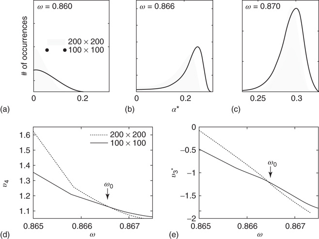
Figure 7.4 Illustration of the dynamics of the 2D torus; the case of KI architecture. There are two distinct dynamic regimes; (a) unimodal pdf with a zero average activation (paramagnetic regime); (b,c) the case of the bimodal pdf with a positive activation level(ferromagnetic regime). (d,e) and around for two graphs of different orders.

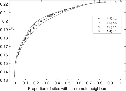
Figure 7.5 Integrated view of the relationship between the proportion of rewired edges and critical noise . Notations 1(1), 1(2), 1(3), and 1(4) mean that a vertex can have 1, 2, 3, or 4 remote connections.

7.4.2 Narrow Band Oscillations in Coupled Excitatory–Inhibitory Lattices

Inhibitory connections in the coupled subgraph can generate oscillations and multimodal activation states [57]. In an oscillator, there are three possible regimes demarcated by two critical points and :

• is the transition point where narrow-band oscillations start.
• is the transition point where narrow-band oscillations terminate.

Under appropriately selected graph parameters, distribution is unimodal when , bimodal when , and quadromodal when , Figure 7.6. Each subgraph has 2304 (5%) edges rewired within the layer and 1728 (3.75%) edges rewired toward the other subgraph. Just below , vertices may oscillate if they are excited. values of temporarily excited graph oscillate, but return to the basal level in the absence of excitation. This form of oscillation is the second building block of neuron-inspired dynamics. When is further increased, that is, , exhibits sustained oscillations even in the absence of external perturbation. When the double layer is temporarily excited, it returns to the basal oscillatory behavior. Self-sustained oscillation is the third building block of neuron-inspired dynamics and it corresponds to KII hierarchy.

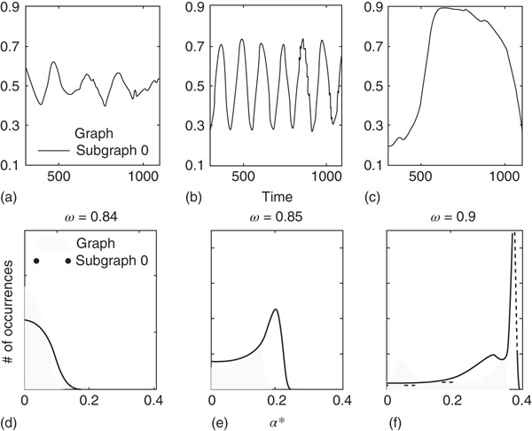
Figure 7.6 Illustration of the dynamics of coupled excitatory–inhibitory layers; the case of KII architecture. There are three modes of the oscillator made of two 2D layers and of order . (a–c) of the whole graph (gray line) and of subgraph (black line) at three different values, which produce three different dynamic modes. (d–e) Distributions of at three different values for graphs of orders and ; only one side of the symmetric distribution is shown.

7.5 BroadBand Chaotic Oscillations

7.5.1 Dynamics of Two Double Arrays

Two coupled layers with inhibitory and excitatory nodes exhibit narrow-band activity oscillations. These coupled lattices with appropriate topology can model any frequency range with oscillations occurring between and . For example, an oscillator has 2.5% edges rewired across the two layers and 5% edges are rewired within each layer. has and , Figure 7.7b. Similarly, oscillator has and . Each of the coupled lattices in this example is of size . When coupling two such oscillators together, we have a total of four layers (tori) coupled into a unified oscillatory system. Clearly, the two oscillators coupled together may or may not agree on a common frequency. We will show that under specific conditions, various operational regimes may occur, including narrow band oscillations, broadband (chaotic) oscillations, intermittent oscillations, and various combinations of these. One of the multiple ways to couple two oscillators is to rewire excitatory edges between subgraphs , -, -, and -, respectively. Two coupled oscillators have additional behavioral regimes. When oscillators and are coupled with 0.625% edges into a new graph , is shifted to lower level, Figure 7.8. Every parameter describing a graph influences the critical behavior under appropriate conditions. If two connected oscillators with different frequencies cannot agree on a common mode, together they can generate large-scale synchronization or chaotic background activity.

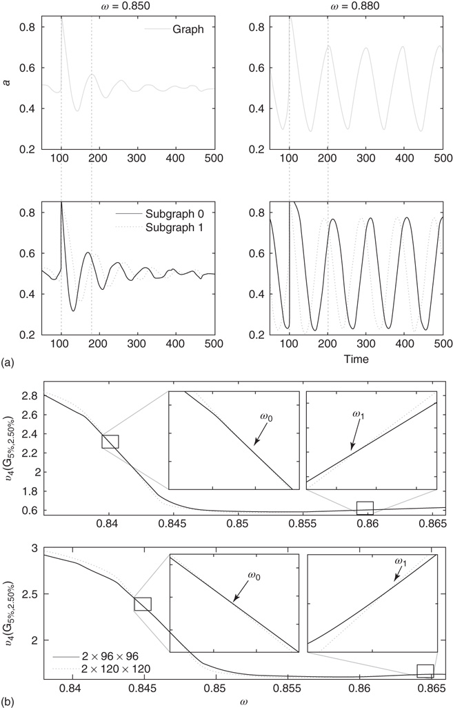
Figure 7.7 Critical states obtained by coupling two double layers of oscillators with rewiring (case of KIII). (a): Left: The graph starts to oscillate after an impulse, but the oscillation decays and returns to the basal level; right: oscillation is sustained even after the input is removed, if . (b): Critical behavior and and values for two different oscillators, (up) and (bottom).

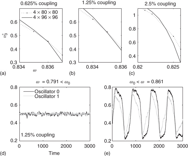
Figure 7.8 Coupling two KII oscillators into KIII, lowers , the point above which large-scale synchronous oscillations are formed. (a–c) values for , , and . (d,e) Typical activation of graph for below and above .

In the graph made of two oscillators, there are four critical points ,separating five possible major operational regimes.

• Case of : The aggregate activation distribution is unimodal and itrepresents the paramagnetic regime in lattice dynamics analogy.
• : The two coupled oscillators exhibit large-scale synchronization and theactivation distribution is bimodal.
• : The two coupled oscillators with different frequencies cannot agree ona common mode, so together they generate aperiodic background activity.
• : Only one oscillator oscillates in a narrow band and the activationdistribution is oktamodal.
• : None of the components exhibit narrow-band oscillation and theactivation distribution is a hexamodal. This corresponds to ferromagnetic state.

These regimes correspond to the fourth building block of neurodynamics, as described by KIII sets.

7.5.2 Intermittent Synchronization of Oscillations in Three Coupled Double Arrays

Finally, we study a system made of three coupled oscillators, each with its own inherent frequency. Such a system produces broadband oscillations with intermittent synchronization–desynchronization behavior. In order to analyze quantitatively the synchronization features of this complex system with over 60 000 nodes in six layers, we merge the channels into a single two-dimensional array at the readout. These channels will be used to measure the synchrony among the graph components. First, we find the dominant frequency of the entire graph using Fourier transform after ensemble averaging across the channels for the duration of the numeric experiment. We set a time window for the duration of two periods determined by the dominant frequency. We calculate the correlation between each channel and the ensemble average over this time window . At each time step, each channel is correlated with the ensemble over the window . Finally, we determine the dominant frequency of each channel and for the ensemble average at time and the phase shifts are calculated. The difference in phases of dominant frequencies measures the phase lag between the channel and the ensemble.

We plot the phase lags across time and space to visualize the synchrony between graph components (see Figure 7.9). We can observe intermittent synchronization spatiotemporal patterns as the function of the , which represents the noise component of the evolution rule. For low values, the phase pattern is unstructured (see Figure 7.9(a)). At a threshold value, intermittent synchronization occurs Figure 7.9b. Further increasing , we reach a regime with highly synchronized channels. Intermittent synchronization across large cortical areas has been observed in ECoG and EEG experiments as well [27, 30]. The correspondence between our theoretical/computational results and experimental data is encouraging. Further detailed studies are needed to identify the significance of the findings.

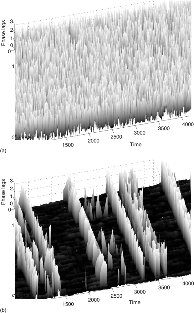
Figure 7.9 Desynchronization to synchronization transitions; (a) at below critical value there is no synchronization; (b) when exceeds a critical value, the graph exhibits intermittent large-scale synchronization.

7.5.3 Hebbian Learning Effects

According to principles of neurodynamics, learning reinforces Hebbian cell assemblies, which respond o known stimuli [16, 23, 24] by destabilizing the broadband chaotic dynamics and lead to an attractor basin through a narrow-band oscillation using gamma band career frequency. To test this model, we implemented learning in the neuropercolation model. We use Hebbian learning, that is, the weight from node i to node j is incrementally increased if these two nodes have the same state or . The weight from i to j incrementally decreases if the two nodes have different activations or . Learning has been maintained during the 20-step periods when input was introduced.

In the basal mode without learning, the three double layers can generate broadband chaotic oscillations; see Figure 7.10a where the lower row is a zoomed-in version of the top row. The spikes in Figure 7.10a indicate the presence of input signals. Inputs have been implemented by flipping a small percentage of the input layer nodes to state “1” (active) for the duration of 20 iteration steps. During the learning stage, inputs are introduced 40 times (20 steps each), at regular intervals of 500 iteration steps. Without learning, the activity returns to the low-level chaotic state soon after the input ceases. Figure 7.10b shows that a narrow-band oscillation becomes prominent during learning, when a specific input is presented. After learning, the oscillatory behavior of the lattice dynamics is more prominent, even without input, but the learnt input elicits much more significant oscillations. This is the manifestation of the sixth and seventh principles of Freeman's neurodynamics, and it can be used to implement classification and control tasks using the neuropercolation model.

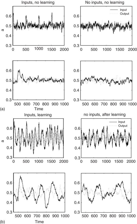
Figure 7.10 Learning effect in coupled oscillators. (a) Activity levels without learning; the first row contains extended time series plots, the second row has zoomed in sections. Input spike is shown at every 500 steps. The activity returns to base level after the input ceases. (b): Activity levels with learning; the oscillations are prominent during learning and maintained even after the input step is removed (decayed).

Further steps, toward the eighth and ninth principles, involve the analysis of the AM pattern, which is converted to a feature vector of dimension . Here, is the number of nodes in our lattice, which, after some course graining, corresponds to the EEG/ECoG electrodes. They provide our observation window into the operation of the cortex or cortex simulation. The feature vector is used to describe or label the cortical state at any moment. The AM pattern is formed by a low-dimensional, quasi-limit cycle attractor after synaptic changes with learning. The synaptic weights are described in a matrix, and the combination of different modalities to form Gestalts is done by concatenation of feature vectors. Research in this direction is in progress.

7.6 Conclusions

We employed the neuropercolation model to demonstrate basic principles of neurodynamics. Neuropercolation is a family of stochastic models based on the mathematical theory of probabilistic CA on lattices and random graphs and motivated by structural and dynamical properties of neural populations. The existence of phase transitions has been demonstrated in probabilistic CA and percolation models. Neuropercolation extends the concept of phase transitions to large interactive populations of nerve cells near criticality. Criticality in the neuropil is characterized by a critical region instead of a singular critical point. The trajectory of the brain as a dynamical system crosses the critical region from a less organized (gaseous) phase to a more organized (liquid) phase during input-induced destabilization and vice versa. Neuropercolation simulates these important results from mesoscopic ECoG/EEG recording across large spatial and temporal scales.

We showed that neuropercolation is able to naturally model input-induced destabilization of the cortex and the consequent phase transitions due to sensory input and learning effects. Broadband activity with scale-free power spectra is observed for unlearnt conditions. On the other hand, Hebbian learning results in the onset of narrow-band oscillations, indicating the selection of specific learnt inputs. These observations demonstrate the operation of the first seven building blocks of neurodynamics. Our results indicate that the introduced Hebbian learning effect can be used to identify and classify inputs. Considering that our model has six coupled lattices, each with up to 10 000 nodes, massive computational resources have been involved in the simulations. Parallel chip implementation may be a natural way to expand the research in the future, especially when extending the work for multisensory Gestalt formation in the cortex.

References

1. 1. von Neumann, J. (1958) The Computer and the Brain, Yale University Press, New Haven, CT.
2. 2. Turing, A. (1954) The chemical basis of morphogenesis. Philos. Trans. R. Soc. London, Ser. B, 237, 37–94.
3. 3. Katchalsky, A. (1971) Biological flow structures and their relation to chemodiffusional coupling. Neurosci. Res. Progr. Bull., 9, 397–413.
4. 4. Prigogine, I. (1980) From Being to Becoming: Time and Complexity in the Physical Sciences, WH Freeman, San Francisco, CA.
5. 5. Haken, H. (1983) Synergetics: An Introduction, Springer-Verlag, Berlin.
6. 6. Haken, H., Kelso, J., and Bunz, H. (1985) A theoretical model of phase transitions in human hand movements. Biol. Cybern., 51, 347–356.
7. 7. Kelso, J. (1995) Dynamic Patterns: The Self-Organization of Brain and Behavior, MIT Press, Cambridge, MA.
8. 8. Haken, H. (2002) Brain Dynamics: Synchronization and Activity Patterns in Pulse-Coupled NeuralNets with Delays and Noise, Springer-Verlag, Heidelberg.
9. 9. Beggs, J.M. and Plenz, D. (2003) Neuronal avalanches in neocortical circuits. J. Neurosci., 23 (35), 11 167.
10. 10. Bak, P. (1996) How Nature Works: The Science of Self-Organized Criticality, Springer-Verlag, New York.
11. 11. Beggs, J. (2008) The criticality hypothesis: how local cortical networks might optimize information processing. Philos. Trans. R. Soc. A Math. Phys. Eng. Sci., 366 (1864), 329–343.
12. 12. Petermann, T., Thiagarajan, T.C., Lebedev, M.A., Nicolelis, M.A.L., Chialvo, D.R., and Plenz, D. (2009) Spontaneous cortical activity in awake monkeys composed of neuronal avalanches. Proc. Natl. Acad. Sci. U.S.A., 106 (37), 15 921.
13. 13. Kozma, R. and Puljic, M. (2005) Phase transitions in the neuropercolation model of neural populations with mixed local and non-local interactions. Biol. Cybern., 92, 367–379.
14. 14. Freeman, W. and Zhai, J. (2009) Simulated power spectral density (PSD) of background electrocorticogram (ECoG). Cogn. Neurodyn., 3 (1), 97–103.
15. 15. Bonachela, J.A., de Franciscis, S., Torres, J.J., and Munoz, M.A. (2010) Self-organization without conservation: are neuronal avalanches generically critical? J. Stat. Mech.: Theory Exp., 2010 (02), P02 015.
16. 16. Freeman, W.J. (1975) Mass Action in the Nervous System, Academic Press, New York.
17. 17. Chang, H. and Freeman, W. (1998a) Biologically modeled noise stabilizing neurodynamics for pattern recognition. Int. J. Bifurcation Chaos, 8 (2), 321–345.
18. 18. Chang, H. and Freeman, W. (1998b) Local homeostasis stabilizes a model of the olfactory system globally in respect to perturbations by input during pattern classification. Int. J. Bifurcation Chaos, 8 (11), 2107–2123.
19. 19. Freeman, W. (1987) Simulation of chaotic EEG patterns with a dynamic model of the olfactory system. Biol. Cybern., 56 (2-3), 139–150.
20. 20. Freeman, W. (1991) The physiology of perception. Sci. Am., 264 (2), 78–85.
21. 21. Freeman, W. (1995) Chaos in the brain: possible roles in biological intelligence. Int. J. Intell. Syst., 10 (1), 71–88.
22. 22. Principe, J., Tavares, V., Harris, J., and Freeman, W. (2001) Design and implementation of a biologically realistic olfactory cortex in analog VLSI. Proc. IEEE, 89, 1030–1051.
23. 23. Freeman, W. (1992) Tutorial on neurodynamics. Int. J. Bifurcation Chaos, 2, 451.
24. 24. Freeman, W. (1999) How Brains Make Up Their Minds, Weidenfeld & Nicolson, London.
25. 25. Kozma, R. (2007) Neuropercolation. Scholarpedia, 2 (8), 1360.
26. 26. Neumann, J.V. and Burks, A. (1966) Theory of Self-Reproducing Automata, University of Illinois Press, Urbana, IL.
27. 27. Freeman, W. (2004) Origin, structure, and role of background EEG activity. Part 1. analytic amplitude. Clin. Neurophysiol., 115 (9), 2077–2088.
28. 28. Kozma, R. and Freeman, W. (2008) Interdispl Intermittent spatio-temporal desynchronization and sequenced synchrony in ECoG signals. Interdispl. J. Chaos, 18, 037 131.
29. 29. Freeman, W. and Kozma, R. (2010) Freeman's mass action. Scholarpedia, 5 (1), 8040.
30. 30. Freeman, W. and Quiroga, Q. (2013) Imaging Brain Function with EEG and ECoG, Springer-Verlag, New York.
31. 31. Freeman, W. and Erwin, H. (2008) Freeman k-set. Scholarpedia, 3 (2), 3238.
32. 32. Chang, H. and Freeman, W. (1998c) Optimization of olfactory model in software to give power spectra reveals numerical instabilities in solutions governed by aperiodic (chaotic) attractors. Neural Networks, 11, 449–466.
33. 33. Kozma, R. and Freeman, W. (2001) Chaotic resonance - methods and applications for robust classification of noisy and variable patterns. Int. J. Bifurcation & Chaos, 11 (6), 1607–1629.
34. 34. Xu, D. and Principe, J. (2004) Dynamical analysis of neural oscillators in an olfactory cortex model. IEEE Trans. Neural Netw., 5 (5), 1053–1062.
35. 35. Ilin, R. and Kozma, R. (2006) Stability of coupled excitatory-inhibitory neural populations and application to control of multi-stable systems. Phys. Lett. A, 360 (1), 66–83.
36. 36. Gutierrez-Osuna, R. and Gutierrez-Galvez, A. (2003) Habituation in the KIII olfactory model with chemical sensor arrays. IEEE Trans. Neural Netw., 14 (6), 1565–1568.
37. 37. Freeman, W., Kozma, R., and Werbos, P. (2001) Biocomplexity: adaptive behavior in complex stochastic systems. BioSystems, 59, 109–123.
38. 38. Beliaev, I. and Kozma, R. (2007) Time series prediction using chaotic neural networks: case study of cats benchmark test. Neurocomputing, 7 (13), 2426–2439.
39. 39. Harter, D. and Kozma, R. (2005) Chaotic neurodynamics for autonomous agents. IEEE Trans. Neural Netw., 16 (3), 565–579.
40. 40. Kozma, R., Aghazarian, H., Huntsberger, T., Tunstel, E., and Freeman, W. (2007) Computational aspects of cognition and consciousness in intelligent devices. IEEE Comput. Intell. Mag., 2 (3), 53–64.
41. 41. Kozma, R., Huntsberger, T., Aghazarian, H., Tunstel, E., Ilin, R., and Freeman, W. (2008) Intentional control for planetary rover SRR2K. Adv. Robot., 21 (8), 1109–1127.
42. 42. Freeman, W. and Vitiello, G. (2008) Dissipation and spontaneous symmetry breaking in brain dynamics. J. Phys. A: Math. Theory, 41, 304 042.
43. 43. Freeman, W., Kozma, R., and Vitiello, G. (2012a) Adaptation of the generalized carnot cycle to describe thermodynamics of cerebral cortex. International Joint Conference on Neural Networks IJCNN2012, 10-15 June, 2012, Brisbane, QLD.
44. 44. Kozma, R. and Puljic, M. (2013) Hierarchical Random Cellular Neural Networks for System-Level Brain-Like Signal Processing. Neural Networks, 45, pp. 101–110.
45. 45. Erds, P. and Rényi, A. (1959) On Random Graphs I, Publicationes Mathematicae, pp. 290–297.
46. 46. Bollobás, B. (1984) The evolution of random graphs. Trans. Am. Math. Soc., 286 (1), 257–274.
47. 47. Bollobas, B. and Riordan, O. (2006) Percolation, Cambridge University Press, New York.
48. 48. Watts, D. and Strogatz, S. (1998) Collective dynamics of “small-world” networks. Nature, 393, 440–442.
49. 49. Sporns, O. (2006) Small-world connectivity, motif composition, and complexity of fractal neuronal connections. BioSystems, 85, 55–64.
50. 50. Berlekamp, E., Conway, J., and Guy, R. (1982) Winning Ways for Your Mathematical Plays: Games in General, Vol. 1, Academic Press, New York.
51. 51. Cipra, A. (1987) An introduction to the Ising model. Am. Math. Mon., 94 (10), 937–959.
52. 52. Marcq, P., Chaté, H., and Manneville, P. (1997) Universality in ising-like phase transitions of lattices of coupled chaotic maps. Phys. Rev. E, 55 (3), 2606–2627.
53. 53. Wolfram, S. (2002) A New Kind of Science, Wolfram Media, Champaign, IL.
54. 54. Balister, P., Bollobás, B., and Kozma, R. (2006) Large deviations for mean field models of probabilistic cellular automata. Random Struct. Algor., 29 (3), 399–415.
55. 55. Kozma, R., Puljic, M., Bollobás, B., Balister, P., and Freeman, W. (2005) Phase transitions in the neuropercolation model of neural populations with mixed local and non-local interactions. Biol. Cybern., 92 (6), 367–379.
56. 56. Binder, K. (1981) Finite size scaling analysis of ising model block distribution functions. Z. Phys. B: Condens. Matter, 43 (2), 119–140.
57. 57. Puljic, M. and Kozma, R. (2008) Narrow-band oscillations in probabilistic cellular automata. Phys. Rev. E, 78 (026214), 6.
58. 58. Ferrenberg, A. and Swendsen, R. (1988) New Monte Carlo technique for studying phase transitions. Phys. Rev. Lett., 61 (23), 2635–2638, doi: 10.1103/PhysRevLett.61.2635.
59. 59. Li, Z., L, S., and B, Z. (1995) Dynamic monte carlo measurement of critical exponents. Phys. Rev. Lett., 74 (17), 3396–3398, doi: 10.1103/PhysRevLett.74.3396.
60. 60. Loison, D. (1999) Binder's cumulant for the Kosterlitz–Thouless transition. Journal of Physics: Condensed Matter, 11 (34), 10.1088/0953-8984/11/34/101.
61. 61. Hasenbusch, M. (2008) The binder cumulant at the Koesterlitz–Thouless transition. Journal of Statistical Mechanics: Theory and Experiment, 2008 (08), P08 003.
62. 62. Kozma, R., Puljic, M., Balister, P., Bollobás, B. and Freeman, W. (2004) Neuropercolation: A random cellular automata approach to spatio-temporal neurodynamics. Lecture Notes in Computer Science, 3305, 435–443.