10
Self-Organized Criticality in Neural Network Models

Matthias Rybarsch and Stefan Bornholdt

10.1 Introduction

Information processing by a network of dynamical elements is a delicate matter: avalanches of activity can die out if the network is not connected enough or if the elements are not sensitive enough; on the other hand, activity avalanches can grow and spread over the entire network and override information processing as observed in epilepsy.

Therefore, it has long been argued that neural networks have to establish and maintain a certain intermediate level of activity in order to keep away from the regimes of chaos and silence [1–4]. Similar ideas were also formulated in the context of genetic networks, where Kauffman postulated that information processing in these evolved biochemical networks would be optimal near the “edge of chaos,” or criticality, of the dynamical percolation transition of such networks [5].

In the wake of self-organized criticality (SOC), it was asked if neural systems were also self-organized to some form of criticality [6]. In addition, actual observations of neural oscillations within the human brain were related to a possible SOC phenomenon [7]. An early example of a SOC model that had been adapted to be applicable to neural networks is the model by Eurich et al. [8]. They show that their model of the random neighbor Olami – Feder–Christensen universality class exhibits (subject to one critical coupling parameter) distributions of avalanche sizes and durations, which they postulate could also occur in neural systems.

Another early example of a model for self-organized critical neural networks [4, 9] drew on an alternative approach to SOC based on adaptive networks [10]. Here, networks are able to self-regulate toward and maintain a critical system state, via simple local rewiring rules that are plausible in the biological context.

After these first model approaches, indeed strong evidence for criticality in neural systems has been found in terms of spatiotemporal activity avalanches, first in the seminal work of Beggs and Plenz [11]. Much further experimental evidence has been found since, which we briefly review below. These experimental findings sparked intense research on dynamical models for criticality and avalanche dynamics in neural networks, which we also give a brief overview subsequently. While most models emphasized biological and neurophysiological detail, our path here is different:

The purpose of this review is to pick up the thread of the early self-organized critical neural network model [4] and test its applicability in the light of experimental data. We would like to keep the simplicity of the first spin model in the light of statistical physics, while lifting the drawback of a spin formulation with respect to the biological system [12]. We will study an improved model and show that it adapts to criticality exhibiting avalanche statistics that compare well with experimental data without the need for parameter tuning [13].

10.2 Avalanche Dynamics in Neuronal Systems

10.2.1 Experimental Results

Let us first briefly review the experimental studies on neuronal avalanche dynamics. In 2003, Beggs and Plenz [11] published their findings about a novel mode of activity in neocortical neuron circuits. During in vitro experiments with cortex slice cultures of the rat, where neuronal activity in terms of local field potentials was analyzed via a multielectrode array, they found evidence of spontaneous bursts and avalanche-like propagation of activity followed by silent periods of various lengths. The observed power-law distribution of event sizes indicates the neuronal network is maintained in a critical state. In addition, they found that the precise spatiotemporal patterns of the avalanches are stable over many hours and also robust against external perturbations [14]. They concluded that these neuronal avalanches might play a central role for brain functions like information storage and processing. Also, during the developmental stages of in vitro cortex slice cultures from newborn rats, neuronal avalanches were found, indicating a homeostatic evolution of the cortical network during postnatal maturation [15]. Moreover, cultures of dissociated neurons were also found to exhibit this type of spontaneous activity bursts in different kinds of networks, as for example in rat hippocampal neurons and leech ganglia [16], as well as dissociated neurons from rat embryos [17].

Aside from these in vitro experiments, extensive studies in vivo have since been conducted. The emergence of spontaneous neuronal avalanches has been shown in anesthetized rats during cortical development [18] as well as in awake rhesus monkeys during ongoing cortical synchronization [19].

The biological relevance of the avalanche-like propagation of activity in conjunction with a critical state of the neuronal network has been emphasized in several works recently. Such network activity has proved to be optimal for maximum dynamical range [20–22], maximal information capacity, and transmission capability [23], as well as for a maximal variability of phase synchronization [24].

10.2.2 Existing Models

The experimental studies with their rich phenomenology of spatiotemporal patterns sparked a large number of theoretical studies and models for criticality and self-organization in neural networks, ranging from very simple toy models to detailed representations of biological functions. Most of them try to capture self-organized behavior with emerging avalanche activity patterns, with scaling properties similar to the experimental power-law event size or duration distributions.

As briefly mentioned earlier, early works as [10] and [4, 9] focus on simple mechanisms for self-organized critical dynamics in spin networks, which also have been discussed in a wider context [25]. These models represent an approach aiming at utmost simplicity of the model, quite similar to the universality viewpoint of statistical mechanics, rather than faithful representations of neurobiological and biochemical detail. Nevertheless, they are able to self-regulate toward and maintain a critical system state, manifested in features as a certain limit cycle scaling behavior, via simple local rewiring rules that are still plausible in the biological context. We take a closer look at these models in Section 10.3, because they provide some of the groundwork for current models.

Regarding neuronal avalanches, a 2002 work by Eurich et al. investigates networks of globally coupled threshold elements that are related to integrate-and-fire neurons. They present a model that, after proper parameter tuning, exhibits avalanche-like dynamics with distinctive distributions of avalanche sizes and durations as expected at a critical system state [8].

It is notable that these models came up even before experimental evidence was found for the existence of neuronal avalanches in [11]. Understandably, extensive studies have been done on avalanche models following their discovery. Again, most models have their mechanisms of self-organization motivated by brain plasticity.

A 2006 model proposed by de Arcangelis et al. consists of a model electrical network on a square lattice, where threshold firing dynamics, neuron refractory inhibition, and activity-dependent plasticity of the synaptic couplings, represented by the conductance of the electrical links, serve as the basis for self-organization. Neuron states are characterized by electrical potentials, which may be emitted as action potentials to neighboring nodes once a certain threshold has been reached. With these incoming currents, the neighbor sites can eventually also reach their activation threshold and thus activity avalanches can propagate through the network. Avalanches are triggered by external currents to specific input sites.Following the activation of a node, the coupling conductances are increased by a small value for each link, which has carried a firing current. On the other hand, after completing a whole avalanche, all couplings in the network have their conductance reduced by the average of the increase that has taken place before, during the avalanche propagation. This way, those couplings that carry many signals will effectively get stronger connections, while the rather inactive connections will be reduced and subsequently pruned from the network. Indeed, the model evolves to a critical state with power-law scaling of avalanche sizes [26]. In a subsequent work, the same behavior of such an adaptive model could also be observed on a class of scale-free networks (namely Apollonian networks), which is argued to be more appropriate as an approach to real neuronal networks than a lattice would be [27].

A related model (in terms of insertion of links or facilitation of weights where signals have been passed) has been proposed by Meisel and Gross [28]. The authors focus on the interplay between activity-driven vs. spike-time-dependent plasticity and link their model to a phase transition in synchronization of the network dynamics. The temporal sequence of node activations serves as the key criterion for the topological updates. While they do not specifically discuss avalanche-like activity patterns, one observes power-law distributed quantities as for example correlation measures or synaptic weights in the self-organized states which point to dynamical criticality.

While the last three models mentioned are set up to strengthen those couplings over which signals have been transmitted, a kind of opposite approach was proposed by Levina et al. [29]. In their model, synaptic depression after propagation of activity over a link – biologically motivated by the depletion of neurotransmitter resources in the synapse – is the key mechanism that drives their model to a critical behavior. The network consists of fully connected integrate-and-fire neurons whose states are described by a membrane potential. This potential is increased by incoming signals from other sites or by random external input, and may cause the site to emit signals when the activation threshold is exceeded. Following such a firing event, the membrane potential is reduced by the threshold value. Again, a single neuron starting to fire after external input, may set off an avalanche by passing its potential to other sites, which in turn can exceed their activation threshold, and so on. The couplings in this model take nondiscrete values, directly related to the biologically relevant amount of neurotransmitter available in each synapse. In short, whenever a signal is passed by a synapse, its value will be decreased. The coupling strength is, on the other hand, recovering slowly toward the maximum value in periods when no firing events occur. The authors also extend the model to consider leaky integrate-and-fire neurons, and find a robust self-organization toward a critical state, again with the characteristic power-law distribution of avalanche sizes. In a later work [30], the authors further investigate the nature of the self-organization process in their model and discuss the combination of first- and second-order phase transitions with a self-organized critical phase.

Meanwhile, field-theoretic approaches to fluctuation effects helped shed light on the universality classes to expect in critical neural networks [31] and the presence of SOC in nonconservative network models of leaky neurons were linked to the existence of alternating states of high versus low activity, so-called up- and down-states [32]. It has been shown that anti-Hebbian evolution is generally capable of creating a dynamically critical network when the anti-Hebbian rule affects only symmetric components of the connectivity matrix. The anti-symmetric component remains as an independent degree of freedom and could be useful in learning tasks [33]. Another model highlights the importance of synaptic plasticity for a phase transition in general and relates the existence of a broad critical regime to a hierarchical modularity [34]. The biological plausibility of activity-dependent synaptic plasticity for adaptive self-organized critical networks has further been stressed recently [35]. Also, the robustness of critical brain dynamics to complex network topologies has been emphasized [36].

The relevance of the critical state in neuronal networks for a brain function as learning was underlined in [37], where the authors find that the performance in learning logical rules as well as time to learn are strongly connected to the strength of plastic adaptation in their model, which at the same time is able to reproduce critical avalanche activity. In a more recent work [38], the same authors present a new variant of their electrical network model. They again use facilitation of active synapses as their primary driving force in the self-organization, but now focus more on activity correlation between those nodes that are actually active in consecutive time steps. Here, they investigate the emergence of critical avalanche events on a variety of different network types, as, for example, regular lattices, scale-free networks, small-world networks, or fully connected networks.

Also, most recently, [39] investigate the temporal organization of neuronal avalanches in real cortical networks. The authors find evidence that the specific waiting time distribution between avalanches is a consequence of the above-mentioned up- and down-states, which in turn is closely linked to a balance of excitation and inhibition in a critical network.

While the proposed organization mechanisms strongly differ between the individual models (see Figure 10.1 for a cartoon representation of the various mechanisms), the resulting evolved networks tend to be part of only a few fundamental universality classes, exhibiting, for example, avalanche statistics in a similar way as in the experimental data, as power-law distributions at an exponent of . With the recent, more detailed models in mind, we are especially interested in the underlying universality of self-organization, also across other fields. Considering the enormous interest in neuronal self-organization, we here come back to our older spin models [4, 10] and develop a new basic mechanism in the light of better biological plausibility of these models.

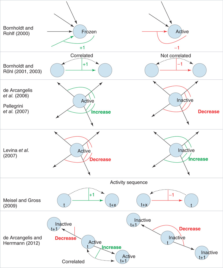
Figure 10.1 Schematic illustration of some of the different approaches to self-organization in neural network models. Rows 1 − 2: Links are either added (denoted by +1; green link) or removed (denoted by −1; red link) as a function of node activity or correlation between nodes. Rows 3 - 4: Here, activity or inactivity of a node affects all outgoings links (thin lines). All weights of the outgoing links from a node are decreased (red) or increased (green) as a function of node activity. Row 5: Links are created and facilitated when nodes become active in the correct temporal sequence. Links directed against the sequence of activation are deleted. Row 6: Positive correlation in the activity between two nodes selectively increases the corresponding link, whereas there is non-selective weight decrease for links between uncorrelated or inactive nodes.

10.3 Simple Models for Self-Organized Critical Adaptive Neural Networks

10.3.1 A First Approach: Node Activity Locally Regulates Connectivity

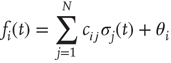
In the very minimal model of a random threshold network [10], a simple local mechanism for topology evolution based on node activity has been defined, which is capable of driving the network toward a critical connectivity of . Consider a network composed of randomly and asymmetrically connected spins (), which are updated synchronously in discrete time steps via a threshold function of the inputs they receive:

10.1

using

10.2

and

10.3

where the link weights have discrete values (or if node does not receive input from node ). In the minimal model, activation thresholds are set to for all nodes. A network run is started with random initial configuration and iterated until either a fixed point attractor or a limit cycle attractor is reached. The attractor of a network is where its dynamics ends up after a while, which is either a fixed point of the dynamics (all nodes reach a constant state) or a limit cycle of the whole network dynamics. A limit cycle in these discrete dynamical models is a cyclic sequence of a finite number of activation patterns.

For the topological evolution, a random node is selected and its activity during the attractor period of the network is analyzed. The network is observed until such an attractor is reached; and afterwards, activity of the single node during that period is measured. In short, if node changes its state at least once during the attractor, a random one of the existing nonzero in-links to that node is removed. If, vice versa, remains constant throughout the attractor period, a new nonzero in-link from a random node is added to the network.

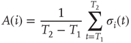
In one specific among several possible realizations of an adaptation algorithm, the average activity of node over an attractor period from to is defined as

10.4

Topological evolution is now imposed in the following way:

1. A random network with average connectivity is created and node states are set to random values.
2. Parallel updates according to Eq. (10.1) are executed until a previous state reappears (i.e., until a dynamical attractor is reached).
3. Calculate for a randomly selected node . If , node receives a new in-link of random weight from a random other node . Otherwise (i.e., if the state of node changes during the attractor period), one of the existing in-links is set to zero.
4. Optional: a random nonzero link in the network has its sign reversed.

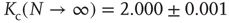
A typical run of this algorithm will result in a connectivity evolution as shown in Figure 10.2 for a network of nodes. Independent of the initial connectivity , the system evolves toward a statistically stationary state with an average evolved connectivity of . With increasing system size , converges toward for the large system limit with a scaling relationship

10.5

with and (compare Figure 10.3).

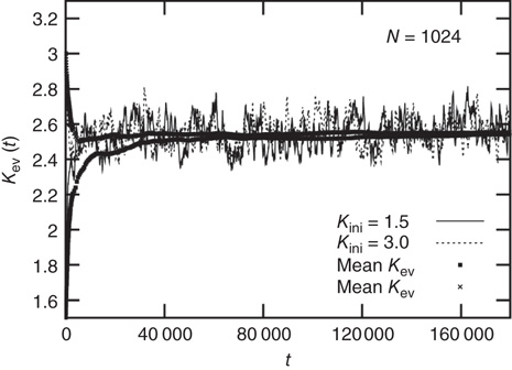
Figure 10.2 Evolution of the average connectivity K_ev with an activity-driven rewiring, shown for two different initial connectivities. Independent of the initial conditions chosen at random, the networks evolve to an average connectivity, 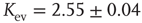. Time t is in simulation steps.

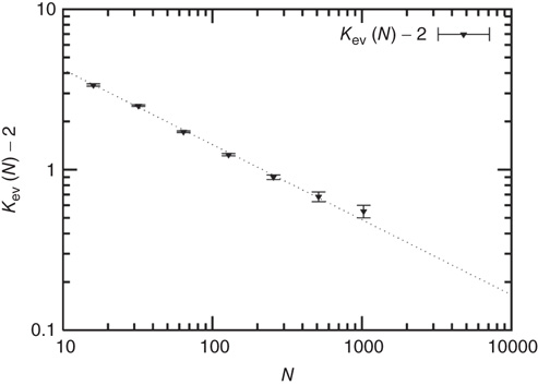
Figure 10.3 A finite-size scaling of the evolved average connectivity K_ev as a function of network size N reveals that for large , the mean converge toward the critical connectivity . For systems with N ≤ 256, the average was taken over 4 × 10⁶ time steps, for N = 512 and N = 1024 over 5 × 10⁵ and 2.5 × 10⁵ time steps respectively.

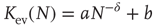
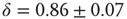
The underlying principle that facilitates self-organization in this model is based on the activity of a node being closely connected to the frozen component of the network – the fraction of nodes which do not change their state along the attractor – which also undergoes a transition from a large to a vanishing frozen component at the critical connectivity. At low network connectivity, a large fraction of nodes will likely be frozen, and thus receive new in-links once they are selected for rewiring. On the other hand, at high connectivity, nodes will often change their state and in turn lose in-links in the rewiring process. Figure 10.4 shows the above-mentioned transition as a function of connectivity for two different network sizes. With a finite-size scaling of the transition connectivities at the respective network sizes, it can be shown that for large , the transition occurs at the critical value of .

Figure 10.4 The frozen component C(K,N) of random threshold networks, as a function of the networks' average connectivities , shown for two different network sizes. Sigmoid function fits can be used for a finite-size scaling of the transition connectivity from active to frozen networks. The results indicate that this transition takes place at for large , details can be found in the original work [10].

10.3.2 Correlation as a Criterion for Rewiring: Self-Organization on a Spin Lattice Neural Network Model

The models described in the following section and originally proposed in [4, 9] capture self-organized critical behavior on a two-dimensional spin lattice via a simple correlation-based rewiring method. The motivation behind the new approach was to transfer the idea of self-organization from [10] to neural networks, thus creating a first self-organized critical neural network model.

In contrast to the activity-regulated model [10] discussed earlier, now:

• the topology is constrained to a squared lattice;
• thermal noise is added to the system;
• link weights take nondiscrete values; and
• activation thresholds may vary from 0.

The model consists of a randomly and asymmetrically connected threshold network of spins (), where links can only be established among the eight local neighbors of any lattice site. The link weights can be activating or inhibiting and are chosen randomly from a uniform distribution 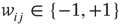. The average connectivity denotes the average number of nonzero incoming weights. All nodes are updated synchronously via a simple threshold function of their input signals from the previous time step:

10.6

with

10.7

and

10.8

where denotes the inverse temperature and is the activation threshold of node . Thresholds are chosen as , where is a small random Gaussian noise of width ε. The model per se exhibits a percolation transition under variation of or , changing between a phase of ordered dynamics, with short transients and limit cycle attractors, and a chaotic phase with cycle lengths scaling exponentially with system size.

On a larger time scale, the network topology is changed by a slow local rewiring mechanism according to the following principle: if the dynamics of two neighboring nodes is highly correlated or anticorrelated, they get a new link between them. Otherwise, if their activity shows low correlation, any present link between them is removed, which is reminiscent of the Hebbian learning rule. In this model, the correlation of nodes over a time interval is defined as

10.9

The full model is constructed as follows:

1. Start with a randomly connected lattice of average connectivity , random initial node configuration, and random individual activation thresholds .
2. Perform synchronous updates of all nodes for time steps. (Here, the choice of τ is not linked to any attractor period measurement, but should be chosen large enough to ensure a separation of time scales between network dynamics and topology changes.)
3. Choose a random node and random neighbor and calculate over the last time steps (a first τ/2 time steps are disregarded to exclude a possible transient period following the previous topology change.)
4. If is larger than a given threshold , a new link from node to is inserted with random weight . If else the weight is set to 0.
5. Use the current network configuration as new initial state and continue with step 2.

Independent of the initial average connectivity , one finds a slow convergence of toward a specific mean evolved connectivity , which is characteristic for the respective network size (Figure 10.5) and shows a finite-size scaling according to

10.10

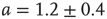with , , and 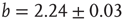, where can be interpreted as the evolved average connectivity for the large system limit :

10.11

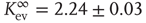
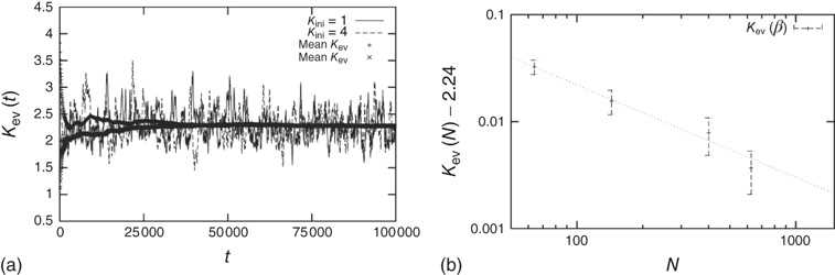
Figure 10.5 (a) Evolution of the average connectivity with a correlation-based rewiring, shown for two different initial connectivities. Again, connectivity evolves to a specific average depending on network size, but independent of the initial configuration. (b) Finite-size scaling of the evolved average connectivity. The best fit is obtained for a large system limit of 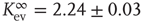. Averages are taken over 4 × 10⁵ time steps.

In addition, it is shown that the proposed adaptation mechanism works robustly toward a wide range of thermal noise , and also the specific choice of the correlation threshold for rewiring only plays a minor role regarding the evolved (Figure 10.6).

Figure 10.6 (a) Evolved average connectivity as a function of the inverse temperature . The behavior is robust over a wide range of . (b) Histogram of the average correlation for a network evolving in time with and . As very low and very high correlations dominate, the exact choice of the correlation threshold during the rewiring process is of minor importance.

Having a closer look at a finite-size scaling of the evolved average attractor length, one finds a scaling behavior close to criticality. While attractor lengths normally scale exponentially with system size in the supercritical, chaotic regime and sublinearly in the subcritical, ordered phase, this model exhibits relatively short attractor cycles also for large evolved networks in the critical regime (Figure 10.7).

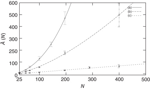
Figure 10.7 Finite-size scaling of the evolved average attractor period (N) for networks of different sizes N (b). Also shown for comparison is the corresponding scaling of the attractor lengths of a supercritical random network (a) with and a subcritical one (c) with .

10.3.3 Simplicity versus Biological Plausibility – and Possible Improvements

10.3.3.1 Transition from Spins to Boolean Node States

In the earlier sections, we have seen that already basic toy models, neglecting a lot of details, can reproduce some of the observations made in real neuronal systems. We now want to move these models a step closer toward biological plausibility and at the same time construct an even simpler model.

One major shortcoming of both models discussed earlier is the fact that they are constructed as spin models. In some circumstances, however, when faithful representation of certain biological details is important, the exact definition matters. In the spin version of a neural network model, for example, a node with negative spin state will transmit nonzero signals through its outgoing weights , despite representing an inactive (!) biological node. In the model, such signals arrive at target nodes , for example, as a sum of incoming signals . However, biological nodes, as genes or neurons, usually do not transmit signals when inactive. Also, in other contexts such as biochemical network models, each node represents whether a specific chemical component is present or absent . Thus, the network itself is mostly in a state of being partially absent as, for example, in a protein network where for every absent protein all of its outgoing links are absent as well. In the spin state convention, this fact is not faithfully represented. A far more natural choice would be to construct a model based on Boolean state nodes, where nodes can be truly “off” () or “on” () – which is precisely what we are going to do in the following sections.

Another example of an inaccurate detail is the common practice of using the standard convention of the Heaviside step function as an activation function in discrete dynamical networks (or the sign function in the spin model context). The convention is not a careful representation of biological circumstances. Both for genes and neurons, a silent input frequently maps to a silent output. Therefore, we use a redefined threshold function defined as

10.12

Most importantly, in our context here, the choice of Boolean node states and the redefined threshold function are vital when we discuss mechanisms of self-organization. For instance, the correlation-based approach presented in the older spin model [4] in Section 10.3.2 explicitly measures contributions by pairs of nodes that could be constantly off () and still treat them as highly correlated (because ) even though there is no activity involved at all. In the later Section 10.3.4, we therefore present a new approach for a network of Boolean state nodes, which does not rely on nonactivity correlations anymore.

10.3.3.2 Model Definitions

Let us consider randomly wired threshold networks of nodes . At each discrete time step, all nodes are updated in parallel according to

10.13

using the input function

10.14

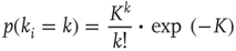
In particular, we choose for plausibility reasons (zero input signal will produce zero output). While the weights take discrete values with equal probability for connected nodes, we select the thresholds for the following discussion. For any node , the number of incoming links is called the in-degree of that specific node. denotes the average connectivity of the whole network. With randomly placed links, the probability for each nodeto actually have incoming links follows a Poissonian distribution:

10.15

10.3.3.3 Exploration of Critical Properties – Activity-Dependent Criticality

To analytically derive the critical connectivity of this type of network model, we first study damage spreading on a local basis and calculate the probability for a single node to propagate a small perturbation, that is, to change its output from 0 to 1 or vice versa after changing a single input state. The calculation can be done closely following the derivation for spin-type threshold networks in Ref. [40], but one has to account for the possible occurrence of “0” input signals also via nonzero links. The combinatorial approach yields a result that directly corresponds to the spin-type network calculation via .

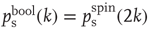However, this approach does not hold true for our Boolean model in combination with the defined theta function as it assumes a statistically equal distribution of all possible input configurations for a single node. In the Boolean model, this would involve an average node activity of over the whole network (where denotes the average fraction of nodes which are active, i.e., ). Instead we find (Figure 10.8) that the average activity on the network is significantly below . At (which will turn out to be already far in the supercritical regime), less than 30% of all nodes are active on average. Around (where we usually expect the critical connectivity for such networks), the average activity is in fact below 10%. Thus, random input configurations of nodes in this network will more likely consist of a higher number of “0” signal contributions than of inputs.

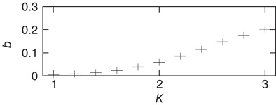
Figure 10.8 Average node activity as function of connectivity measured on attractors of 10 000 sample networks each, 200 nodes.

Therefore, when counting input configurations for the combinatorial derivation of , we need to weight all relevant configurations according to their realization probability as given by the average activity – the detailed derivation can be found in [12]. With the average probability of damage spreading, we can further compute the branching parameter or sensitivity and apply the annealed approximation [10, 41] to obtain the critical connectivity by solving

10.16

However, now depends on the average network activity, which in turn is a function of the average connectivity itself as shown in Figure 10.8.

From the combined plot in Figure 10.9, we find that both curves intersect at a point where the network dynamics – as a result of the current connectivity – exhibit an average activity, which in turn yields a critical connectivity that exactly matches the given connectivity. This intersection thus corresponds to the critical connectivity of the present network model.

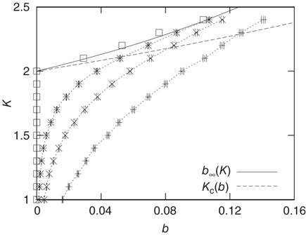
Figure 10.9 Average activity on attractors of different network sizes (right to left: , ensemble averages were taken over 10 000 networks each). Squares indicate activity on an infinite system determined by finite-size scaling, which is in good agreement with the analytic result (solid line). The dashed line shows the analytic result for from Eq. (10.16). The intersections represent the value of for the given network size.

However, the average activity still varies with different network sizes, which is obvious from Figure 10.9. Therefore, the critical connectivity is also a function of . For an analytic approach to the infinite size limit, it is possible to calculate the average network activity at the next time step in an iterative way from the momentary average activity . Again, the details can be found in [12]. We can afterwards distinguish between the different dynamical regimes by solving 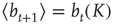for the critical line. The solid line in Figure 10.9 depicts the evolved activity in the long time limit. We find that for infinite system size, the critical connectivity is at

while up to this value all network activity vanishes in the long time limit (). For any average connectivity , a certain fraction of nodes remains active. In finite-size systems, both network activity evolution and damage propagation probabilities are subject to finite-size effects, thus increasing to a higher value.

Finally, let us have a closer look on the average length of attractor cycles and transients. As shown in Figure 10.10, the behavior is strongly dependent on the dynamical regime of the network. As expected and in accordance with early works on random threshold networks [42] as well as random Boolean networks [43], we find an exponential increase of the average attractor lengths with network size in the chaotic regime (), whereas we can observe a power-law increase in the frozen phase (). We find similar behavior for the scaling of transient lengths (inset of Figure 10.10).

Figure 10.10 verage attractor length at different network sizes. Ensemble averages were taken over 10 000 networks each at (a) , (b) , (c) . Inset figure shows the scaling behavior of the corresponding transient lengths.

10.3.3.4 Extension of the Model: Thermal Noise

As is clear from Eq. (10.13), nodes in our model will only switch to active state if they get a positive input from somewhere. Thus, to get activity into the system, we could either define certain nodes to get an additional external input, but this would at the same time create two different kinds of nodes, those with and those without external activity input, which would in turn diminish the simplicity of our model. That is why we will alternatively use thermal noise to create activity, using a Glauber update of the nodes in the same way as it was discussed in the spin model [4] in Section 10.3.2, with one slight modification. We define a probability for the activation of a node, which is a sigmoid function of the actual input sum, but also leaving room for a spontaneous activation related to the inverse temperature of the system.

10.17

with

10.18

and

10.19

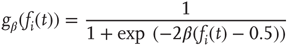
You will note the similarity to the older spin model [4], but be aware that in Eq. (10.18) we shift the input sum by , and we will explain now why this is necessary. Remember that we use binary coupling weights for existing links in our model. The input sum to any node will therefore be an integer value. If we would not shift the input sum, a node with an input (which should always be inactive in the deterministic model without thermal noise), would, after the introduction of the Glauber update rule with nonzero temperature, always have a probability of to be activated, regardless of the actual inverse temperature . Figure 10.11 illustrates this problem. A simple shift of will now give us the desired behavior: Nodes with input will stay off in most cases, with a slight probability to turn active depending on temperature, and, on the other hand, nodes with activating input will be on in most cases, with slight probability to remain inactive. With this modification of the original basic model [12], we can now continue to make our network adaptive and critical.

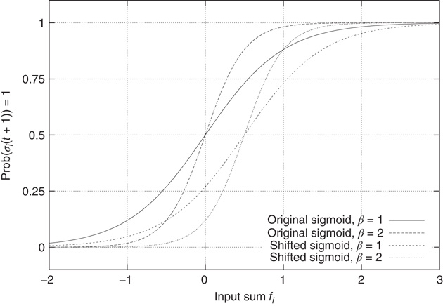
Figure 10.11 With integer input sum values, nodes without input would turn active with probability regardless of temperature. To prevent this, we shift the input sum by such that the transition between off and on state happens exactly in the middle between input sums 0 respectively 1.

10.3.4 Self-Organization on the Boolean State Model

We now want to set up an adaptive network based on the model discussed earlier, which is still capable of self-regulation toward a critical state despite being simplified to the most minimal model possible. Particularly, we want it to

• have a simple, yet biologically plausible rewiring rule, which only uses local information accessible to individual nodes;
• work independently from a special topology as a lattice.

We have already pointed out the problems of a spin formulation of neural network models similar to [4], and possible ways out with the Boolean state model. As a major advantage of the latter, activity avalanches intrinsically occur in this type of network, whereas spin networks typically exhibit continuous fluctuations with no avalanches directly visible. However, the old correlation-based rewiring mechanism will no longer work when inactive nodes are now represented by “” instead of “.” A solution is presented below.

A second aspect that needs to be addressed concerning the self-organization mechanism is topological invariance of the algorithm. The older, correlation-based mechanism from the spin model relies on randomly selecting neighboring sites on a lattice for the rewiring processes. On a lattice, the number of possible neighbors is strictly limited, but on a large random network near critical connectivity, there arefar more unconnected pairs of nodes than there are connected pairs. Thus, randomly selecting pairs of nodes for rewiring would introduce a strong bias toward connecting nodes that were previously unconnected. This results in a strong increase of connectivity and makes a self-organized adaptation toward a critical state practically impossible. If we want to overcome the restriction of, for example, a confined lattice topology in order to improve biological applicability of the model, we have to adapt the rewiring mechanism such that this bias no longer exists.

Of course, the new model shall inherit several important features from the older spin models, which already underline the applicability to biological networks: in particular, it must be capable of self-regulation toward a critical state despite being simplified to the most minimal model possible. The organization process, however, should be based on a simple, yet biologically plausible rewiring rule, which only uses local information accessible to individual nodes like pre- and postsynaptic activity and correlation of such activity.

This section is directly based on our recent work [13].

10.3.4.1 Model Definitions

Consider a randomly connected threshold network of the type discussed in Section 10.3.3. The network consists of nodes of Boolean states , which can be linked by asymmetric directed couplings . Node pairs that are not linked have their coupling set to , and links may exist between any two nodes; so, there is no underlying spatial topology in this model.

All nodes are updated synchronously in discrete time steps via a simple threshold function of their input signals with a little thermal noise introduced by the inverse temperature , in the same way as in the model of Bornholdt and Roehl (Section 10.3.2), but now with an input shift of in the Glauber update, representing the new function as discussed in Section 10.3.3.4:

10.20

with

10.21

and

10.22

For the simplicity of our model, we first assume that all nodes have an identical activation threshold of .

10.3.4.2 Rewiring Algorithm

The adaptation algorithm is now constructed in the following way: we start the network at an arbitrary initial connectivity and do parallel synchronous updates on all nodes according to Eq. (10.16). All activity in this model originates from small perturbations by thermal noise, leading to activity avalanches of various sizes. In this case, we set the inverse temperature to . On a larger time scale, that is, after updates, a topology rewiring is introduced at a randomly chosen, single node. The new element in our approach is to test whether the addition or the removal of one random in-link at the selected node will increase the average dynamical correlation to all existing inputs of that node. By selecting only one single node for this procedure, we effectively diminish the bias of selecting mostly unconnected node pairs – but retain the biologically inspired idea for a Hebbian, correlation-based rewiring mechanism on a local level.

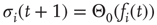
Now, we have to define what is meant by dynamical correlation in this case. We here use the Pearson correlation coefficient to first determine the dynamical correlation between a node and one of its inputs :

10.23

where and in the denominator depict the standard deviation of states of the nodes and , respectively. In case one or both of the nodes are frozen in their state (i.e., yield a standard deviation of 0), the Pearson correlation coefficient would not be defined, we will assume a correlation of . Note that we always usethe state of node at one time step later than node , thereby taking into account the signal transmission time of one time step from one node to the next one. Again, as in the model of [4], the correlation coefficient is only taken over the second half of the preceding time steps in order to avoid transient dynamics. Finally, we define the average input correlation of node as

10.24

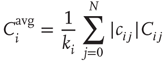
where is the in-degree of node . The factor ensures that correlations are only measured where links are present between the nodes. For nodes without any in-links (), we define .

In detail, the adaptive rewiring is now performed in the following steps:

• Select a random node and generate three clones of the current network topology and state:
  • [Network 1:] This copy remains unchanged.
  • [Network 2:] In this copy, node will get one additional in-link from a randomly selected other node which is not yet connected to in the original copy (if possible, i.e., ). Also, the coupling weight of the new link is chosen at random.
  • [Network 3:] In the third copy, one of the existing in-links to node (again if possible, i.e., ) will be removed.
• All three copies of the network are individually run for time steps.
• On all three networks, the average input correlation of node to all of the respective input nodes in each network is determined.
• We accept and continue with the network which yields the highest absolute value of , the other two clones are dismissed. If two or more networks yield the same highest average input correlation such that no explicit decision is possible, we simply continue with the unchanged status quo.
• A new random node is selected and the algorithm starts over with step 1.

It is worth noting that this model – in the same way as the earlier work by Bornholdt and Röhl [4] – uses locally available information at synapse level and takes into account both pre- and postsynaptic activity (Figure 10.12). This is a fundamental difference to approaches discussed, for example, by de Arcangelis et al. [26–29], where only presynaptic activity determines changes to the coupling weights. Note that the non-locality of running three network copies in parallel that we use here is not critical. A local implementation is straightforward, locally estimating the order parameter (here the average input correlation C_i^avg) as time average, with a sufficient time scale separation towards the adaptive changes in the network. A local version of the model will be studied in the published version of [13].

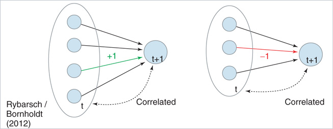
Figure 10.12 Schematic illustration of the rewiring mechanism based on average input correlation. In this example, the target node initially has three in-links. Left: If the addition of a fourth input increases the average input correlation C_i^avg, a link will be inserted. Right: If removal of an existing in-link increases C_i^avg, the link will be deleted.

10.3.4.3 Observations

In the following, we take a look at different observables during numerical simulations of network evolution in the model presented earlier. Key figures include the average connectivity and the branching parameter (or sensitivity) . Both are closely linked to and influenced by the ratio of activating links , which is simply the fraction of positive couplings among all existing (non-zero) links.

Figure 10.13a shows an exemplary run of the topology evolution algorithm, where we start with completely isolated nodes without any links. Trivially, the “network” is subcritical at this stage, which can be seen from the branching parameter which is far below 1. As soon as rewiring takes place, the network starts to insert new links, obviously because these links enable the nodes to pass signals and subsequently act in a correlated way. With increasing connectivity, the branching parameter also rises, indicating that perturbations start to spread from their origin to other nodes. When the branching parameter approaches 1, indicating that the network reaches a critical state, the insertion of new links is cut back. The processes of insertion and depletion of links tend to be balanced against each other, regulating the network close to criticality.

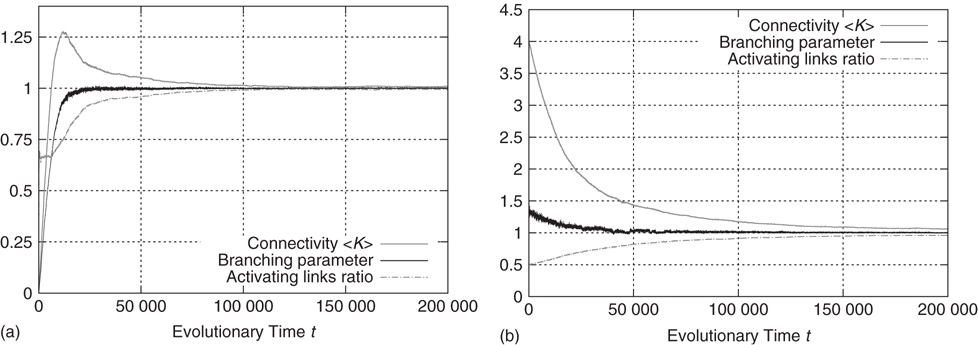
Figure 10.13 Regardless of initial connectivity and sensitivity, the network evolves to a critical configuration. (a) Starting with completely disconnected nodes and obviously subcritical “network.” (b) Starting with a supercritical network.

If we, on the other hand, start with a randomly interconnected network at a higher connectivity like as shown in Figure 10.13b, we find the network in the supercritical regime () at the beginning. When above the critical threshold, many nodes will show chaotic activity with very low average correlation to their respective inputs. The rewiring algorithm reacts in the appropriate way by deleting links from the network, until the branching parameter approaches 1.

In both the above-mentioned examples, the evolution of the ratio of activating links (which tends toward 1) shows that the rewiring algorithm in general favors the insertion of activating links and, vice versa, the deletion of inhibitory couplings. This appears indeed plausible if we remind ourselves that the rewiring mechanism optimizes the inputs of a node toward high correlation, on average. Also, nodes will only switch to active state if they get an overall positive input. As we had replaced spins by Boolean state nodes, this can only happen via activating links – and that is why correlations mainly originate from positive couplings in our model. As a result, we observe the connectivity evolving toward one in-link per node, with the ratio of positive links also tending toward one.

For a richer pattern complexity, we might later want to introduce a second mechanism that balances out positive via negative links, and with a first approach we can already test how the rewiring strategy would fit to that situation: if after each rewiring step, we change the sign of single random links as necessary to obtain a ratio of e.g. 80% activating links (i.e. p =0.8), keeping the large majority of present links unchanged, the branching parameter will again stabilize close to the critical transition, while the connectivity is maintained at a higher value. Figure 10.14 shows that the self-organization behavior is again independent from the initial conditions. This result does not depend on the exact choice of the activating links ratio p; similar plots can easily be obtained for a large range starting at p = 0.5, where the connectivity will subsequently evolve towards a value slightly below , which is the value we would expect as the critical connectivity for a randomly wired network with balanced link ratio according to the calculations made in Section 10.3.3 for the basic network model [12].

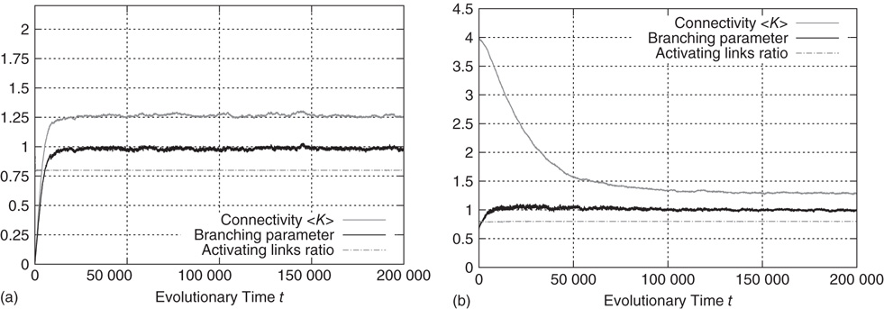
Figure 10.14 Network evolution with activating links ratio kept at p = 0.8.

In addition to the branching parameter measurement, we also take a look at some dynamical properties of the evolved networks to further verify their criticality. As stated in section 10.1, we are especially interested in the resulting activity avalanches on the networks. Figure 10.15a shows the cumulative distribution of avalanche sizes in an evolved sample network of nodes. We observe a broad distribution of avalanche sizes and a power-law-like scaling of event sizes with an exponent close to , corresponding to an exponent of in the probability density – which is characteristic of a critical branching process. At the same time, this is in perfect agreement with the event size distribution observed by Beggs and Plenz in their in vitro experiments.

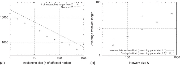
Figure 10.15 (a) Cumulative distribution of avalanche sizes in an evolved sample network of nodes. We find a broad, near power-law distribution comparable to a slope of , indicative of a critical branching process and corresponding well to the experimental results of Beggs and Plenz. (b) Scaling of average transient lengths at different network sizes, 50 evolved networks each.

In our most recent version of [13] we were also able to quantify the scaling behavior of avalanche durations in addition to the size distributions, as well as the relations between durations and spatial sizes of avalanches. We find good agreement of the corresponding scaling exponents with relations predicted by universal scaling theory [44]. and observe avalanche statistics and collapsing avalanche profiles compatible with recent results from biological experiments by Friedman et al [45].

If we randomly activate small fractions of nodes in an otherwise silent network (single nodes up to 5% of the nodes) to set off avalanches, we can also see (Figure 10.15b) that the resulting transient length shows a power-law scaling with network size right up to network snapshots taken after an evolution run at the final average branching parameter of 1. Intermediate networks taken from within an evolution process at a higher branching parameter instead show a superpolynomial increase of transient lengths with system size, which is precisely what we expect.

10.3.5 Response to External Perturbations

In recent in vitro experiments, Plenz [46] could further demonstrate that cortical networks can self-regulate in response to external influences, retaining their functionality, while avalanche-like dynamics persist – for example, after neuronal excitability has been decreased by adding an antagonist for fast glutamatergic synaptic transmission to the cultures.

To reproduce such behavior in our model, we can include variations in the activation thresholds of the individual nodes, which had been set to zero in the above-mentioned discussions for maximum model simplicity. Assume that we start our network evolution algorithm with a moderately connected, but subcritical network, where all nodes have a higher activation threshold of . According to the update rule (10.7), now at least two positive inputs are necessary to activate a single node. As the rewiring algorithm is based on propagation of thermal noise signals, the inverse temperature needs to be selected at a lower value than before. (As a general rule, should be selected in a range where thermal activation of nodes occur at a low rate, such that avalanches can be triggered, but are not dominated by noise.)

Figure 10.16 shows that, same as earlier, the subcritical network starts to grow new links, thereby increasing the average branching parameter. Again, this process is stopped after the supercritical regime is reached. While the system does not approach to a phase transition as well as shown above for activation thresholds of 0 (in fact, the branching fluctuates much more around the target value of 1), the general tendency remains: the rewiring mechanism reacts properly as the network drifts too far off from criticality. At one time step in the center of Figure 10.16, we suddenly reset all nodes to an activation threshold of , simulating the addition of a stimulant. As we can expect, this immediately puts the network into a supercritical, chaotic state. This is reflected by the branching parameter, which now constantly stays above 1 and does not fluctuate below anymore. It is clearly visible that the rewiring mechanism promptly reacts and drives back the connectivity, until the branching parameter slowly converges toward 1 again. A similar behavior is also found if thresholds are not changed all at once, but gradually during network evolution.

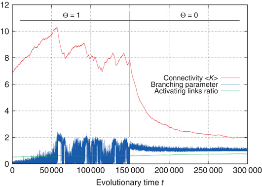
Figure 10.16 Rewiring response to a sudden decrease of activation thresholds. All were set from 1 to 0 in the same time step.

10.4 Conclusion

We have seen that very minimalistic binary neural network models are capable of self-organized critical behavior. While older models show some drawbacks regarding biological plausibility originating directly from their nature as spin networks, we subsequently presented a possible transition to a self-organized critical, randomly wired network of Boolean node states with emerging dynamical patterns, namely, activity avalanches, reminiscent of activity modes as observed in real neuronal systems. This is possible via a simple, locally realizable, rewiring mechanism that uses activity correlation as its regulation criterion, thus retaining the biologically inspired rewiring basis from the spin version. While it is obvious that there are far more details involved in self-organization of real neuronal networks – some of which are reflected in other existing models – we here observe a fundamental organization mechanism leading to a critical system that exhibits statistical properties pointing to a larger class of universality, regardless of the details of a specific biological implementation.

Acknowledgments

For the presentation of the earlier work from our group (Sections 10.3.1 and 10.3.2), excerpts from the text and figures of the original publications [4, 10] were used, as well as from [12, 13] for our recent work.

References

1. 1. Langton, C.G. (1990) Computation at the edge of chaos. Physica D, 42, 12–37.
2. 2. Herz, A.V.M. and Hopfield, J.J. (1995) Earthquake cycles and neural reverberations: collective oscillations in systems with pulse-coupled threshold elements. Phys. Rev. Lett., 75 (6), 1222–1225.
3. 3. Bak, P. and Chialvo, D.R. (2001) Adaptive learning by extremal dynamics and negative feedback. Phys. Rev. E, 63 (3), 031912.
4. 4. Bornholdt, S. and Röhl, T. (2003) Self-organized critical neural networks. Phys. Rev. E, 67 (066118).
5. 5. Kauffman, S. (1993) The Origins of Order: self-Organization and Selection in Evolution, Oxford University Press.
6. 6. Bak, P., Tang, C., and Wiesenfeld, K. (1988) Self-organized criticality. Phys. Rev. A, 38 (1), 364.
7. 7. Linkenkaer-Hansen, K., Nikouline, V.V., Palva, J.M., and Ilmoniemi, R.J. (2001) Long-range temporal correlations and scaling behavior in human brain oscillations. J. Neurosci., 21 (4), 1370–1377.
8. 8. Eurich, C.W., Herrmann, J.M., and Ernst, U.A. (2002) Finite-size effects of avalance dynamics. Phys. Rev. E, 66, 066137.
9. 9. Bornholdt, S. and Röhl, T. (2001) Self-organized critical neural networks. arXiv:cond-mat/0109256v1.
10. 10. Bornholdt, S. and Rohlf, T. (2000) Topological evolution of dynamical networks: Global criticality from local dynamics. Phys. Rev. Lett., 84 (26), 6114–6117.
11. 11. Beggs, J.M. and Plenz, D. (2003) Neuronal avalanches in neocortical circuits. J. Neurosci., 23 (35), 11167–11177.
12. 12. Rybarsch, M. and Bornholdt, S. (2012) Binary threshold networks as a natural null model for biological networks. Phys. Rev. E, 86, 026114.
13. 13. Rybarsch, M. and Bornholdt, S. (2012) A minimal model for self-organization to criticality in binary neural networks. arXiv:1206.0166.
14. 14. Beggs, J.M. and Plenz, D. (2004) Neuronal avalanches are diverse and precise activity patterns that are stable for many hours in cortical slice cultures. J. Neurosci., 24, 5216–5229.
15. 15. Stewart, C.V. and Plenz, D. (2007) Homeostasis of neuronal avalanches during postnatal cortex development in vitro. J. Neurosci. Methods, 169 (2), pp. 405–416.
16. 16. Mazzoni, A., Broccard, F.D., Garcia-Perez, E., Bonifazi, P., Ruaro, M.E., and Torre, V. (2007) On the dynamics of the spontaneous activity in neuronal networks. PLoS One, 2 (5), Article e439.
17. 17. Pasquale, V., Massobrio, P., Bologna, L.L., Chiappalone, M., and Martinoia, S. (2008) Self-organization and neuronal avalanches in networks of dissociated cortical neurons. Neuroscience, 153 (4), 1354-1369.
18. 18. Gireesh, E.D. and Plenz, D. (2008) Neuronal avalanches organize as nested theta- and beta/gamma-oscillations during development of cortical layer 2/3. Proc. Nat. Acad. Sci. U.S.A., 105 (21), 7576–7581.
19. 19. Petermann, T., Thiagarajan, T.C., Lebedev, M.A., Nicolelis, M.A.L., Chialvo, D.R., and Plenz, D. (2009) Spontaneous cortical activity in awake monkeys composed of neuronal avalanches. Proc. Natl. Acad. Sci. U.S.A., 106 (37), 15921-15926.
20. 20. Kinouchi, O. and Copelli, M. (2006) Optimal dynamical range of excitable networks at criticality. Nat. Phys., 2, 348–352.
21. 21. Shew, W.L., Yang, H., Petermann, T., Roy, R., and Plenz, D. (2009) Neuronal avalanches imply maximum dynamic range in cortical networks at criticality. J. Neurosci., 29 (49), 15595–15600.
22. 22. Larremore, D.B., Shew, W.L., and Restrepo, J.G. (2011) Predicting criticality and dynamic range in complex networks: Effects of topology. Phys. Rev. Lett., 106 (5), 058101.
23. 23. Shew, W.L., Yang, H., Yu, S., Roy, R., and Plenz, D. (2011) Information capacity and transmission are maximized in balanced cortical networks with neuronal avalanches. J. Neurosci., 31 (1), 55–63.
24. 24. Yang, H., Shew, W.L., Roy, R., and Plenz, D. (2012) Maximal variability of phase synchrony in cortical networks with neuronal avalanches. J. Neurosci., 32 (3), 1061-1072.
25. 25. Gross, T., and Blasius, B., (2008) Adaptive coevolutionary networks: a review. J. R. Soc. Interface, 5 (20), 259–271.
26. 26. de Arcangelis, L., Perrone-Capano, C., and Herrmann, H.J. (2006) Self-organized criticality model for brain plasticity. Phys. Rev. Lett., 96 (2), 028107.
27. 27. Pellegrini, G.L., de Arcangelis, L., Herrmann, H.J., and Perrone-Capano, C. (2007) Activity-dependent neural network model on scale-free networks. Phys. Rev. E, 76 (1 Pt 2), 016107.
28. 28. Meisel, C., and Gross, T., (2009) Adaptive self-organization in a realistic network model. Phys. Rev. E, 80 (2), 061917.
29. 29. Levina, A., Herrmann, J.M., and Geisel, T. (2007) Dynamical synapses causing self-organized criticality in neural networks. Nat. Phys., 3, 857–860.
30. 30. Levina, A., Herrmann, J.M., and Geisel, T. (2009) Phase transitions towards criticality in a neural system with adaptive interactions. Phys. Rev. Lett., 102 (11), 118110.
31. 31. Buice, M.A. and Cowan, J.D. (2007) Field-theoretic approach to fluctuation effects in neural networks. Phys. Rev. E, 75 (5 Pt 1), 051919.
32. 32. Millman, D., Mihalas, S., Kirkwood, A., and Niebur, E. (2010) Self-organized criticality occurs in non-conservative neuronal networks during ‘up’ states. Nat. Phys., 6, 801–805.
33. 33. Magnasco, M.O., Piro, O., and Cecchi, G.A. (2009) Self-tuned critical anti-hebbian networks. Phys. Rev. Lett., 102, 258102.
34. 34. Rubinov, M., Sporns, O., Thivierge, J.-P., and Breakspear, M. (2011) Neurobiologically realistic determinants of self-organized criticality in networks of spiking neurons. PLoS Comput. Biol., 7 (6), e1002038.
35. 35. Droste, F., Do, A.-L., and Gross, T. (2013) Analytical investigation of self-organized criticality in neural networks. J. R. Soc. Interface., 10 (78).
36. 36. Larremore, D.B., Carpenter, M.Y., Ott, E., and Restrepo, J.G. (2012) Statistical properties of avalanches in networks. Phys. Rev. E, 85, 066131.
37. 37. de Arcangelis, L. and Herrmann, H.J. (2010) Learning as a phenomenon occurring in a critical state. Proc. Natl. Acad. Sci. U.S.A., 107 (9).
38. 38. de Arcangelis, L. and Herrmann, H.J. (2012) Activity-dependent neuronal model on complex networks. Front. Physio., 3 (62).
39. 39. Lombardi, F., Herrmann, H.J., Perrone-Capano, C., Plenz, D., and de Arcangelis, L. (2012) The balance between excitation and inhibition controls the temporal organization of neuronal avalanches. Phys. Rev. Lett., 108, 228703.
40. 40. Rohlf, T. and Bornholdt, S. (2002) Criticality in random threshold networks: annealed approximation and beyond. Physica A, 310, 245–259.
41. 41. Derrida, B. and Pomeau, Y. (1986) Random networks of automata: a simple annealed approximation. Europhys. Lett., 1, 45–49.
42. 42. Kürten, K. (1988) Critical phenomena in model neural networks. Phys. Lett. A, 129 (3), 157–160.
43. 43. Bastolla, U. and Parisi, G. (1996) Closing probabilities in the kauffman model: an annealed computation. Physica D, 98, 1–25.
44. 44. Sethna, J.P., Dahmen, K.A., and Myers, C.R. (2001) Crackling Noise. Nature, 410, 242–250.
45. 45. Friedman, N., Ito, S., Brinkman, B.A.W., Shimono, M., DeVille, R.E.L., Dahmen, K.A., Beggs, J.M., and Butler, T.C. (2012) Universal critical dynamics in high resolution neuronal avalanche data. Phys. Rev. Lett., 108, 208102.
46. 46. Plenz, D. (2012) Neuronal avalanches and coherence potentials. Eur. Phys. J. Special Topics, 205, pp. 259–309.