12
Activity Dependent Model for Neuronal Avalanches

Lucilla de Arcangelis and Hans J. Herrmann

Cortical networks exhibit diverse patterns of spontaneous neural activity, including oscillations, synchrony, and waves. The spontaneous activity, often, in addition exhibits slow alternations between high activity periods, or bursts, followed by essentially quiet periods. Bursts can last from a few to several hundred milliseconds and, if analyzed at a finer temporal scale, show a complex structure in terms of neuronal avalanches. As discussed in the previous chapters, neuronal avalanches exhibit dynamics similar to that of self-organized criticality (SOC), see [1–4]. Avalanches have been observed in organotypic cultures from coronal slices of rat cortex [5], where neuronal avalanches are stable for many hours [6]. The size and duration of neuronal avalanches follow power law distributions with very stable exponents, typical features of a system in a critical state, where large fluctuations are present and system responses do not have a characteristic size. The same critical dynamics has been measured also in vivo in rat cortical layers during early postnatal development [7], in the cortex of awake adult rhesus monkeys [8], as well as in dissociated neurons from rat hippocampus [9, 10] or leech ganglia [9]. The term “SOC” usually refers to a mechanism of slow energy accumulation and fast energy redistribution driving the system toward a critical state, where the distribution of avalanche sizes obeys a power law obtained without fine-tuning of a particular model parameter. The simplicity of the mechanism at the basis of SOC suggests that many physical and biological phenomena characterized by power laws in the size distribution might represent natural realizations of SOC. For instance, SOC has been proposed to model earthquakes [11, 12], the evolution of biological systems [13], solar flare occurrences [14], fluctuations in confined plasma [15], snow avalanches [16], and rain fall [17].

While sizes and durations of avalanches have been intensively studied in neuronal systems, the quiet periods between neuronal avalanches are much less understood. In vitro preparations exhibit such quiescent periods, often called down-states which can last up to several seconds, in contrast to periods of avalanche activity, which generally are shorter in duration. The emergence of these downstates be attributed to a variety of mechanisms: a decrease in the neurotransmitter released by each synapse, either due to the exhaustion of available synaptic vesicles or to the increase of a factor inhibiting the release [18] such as the nucleoside adenosine [19]; the blockage of receptor channels by the presence, for instance, of external magnesium [20]; or else spike adaptation [21]. A downstate is therefore characterized by a disfacilitation, that is, reduction of synaptic activity, indicative of a large number of neurons with long-lasting return to their resting membrane potentials [22]. It was shown analytically and numerically, and discussed in the previous chapters, that self-organized critical behavior characterizes upstates, whereas subcritical behavior characterizes downstates [23].

Here we discuss a neural network model based on SOC ideas that takes into account synaptic plasticity. Synaptic plasticity is one of the most astonishing properties of the brain, occurring mostly during development and learning [24–26]. It is defined as the ability to modify the structural and functional properties of synapses in response to past activity in the network. Such modifications in the strength of synapses are thought to underlie memory and learning. Among the postulated mechanisms of synaptic plasticity, the activity-dependent Hebbian plasticity constitutes the most developed and influential model of how information is stored in neural circuits [27–29]. In order to get real insights into the relation between macroscopic network dynamics and the microscopic, that is, cellular, interactions inside a neural network, it is necessary to identify the basic ingredients of brain activity that could be responsible for characteristic scale-free behavior such as observed for neuronal avalanches. These insights are the basis for any further understanding of the diverse additional features, such as the interpretation by practitioners of electroencephalography (EEG) time series for diagnosis or the understanding of learning behavior. Therefore, the formulation of a neuronal network model that yields the correct scaling behavior for spontaneous activity is of crucial importance for any further progress in the understanding of the living brain.

12.1 The Model

In order to formulate a new model to study neuronal activity, we incorporated [30, 31] into a SOC framework three important neuronal ingredients, namely action potential firing after the neuronal intracellular membrane potential reaches a threshold, the refractory period of a neuron after firing an action potential, and activity-dependent synaptic plasticity. We consider a lattice of sites where each site represents the cell body of a neuron and each bond a synaptic connection to a neighboring neuron. Each neuron is characterized by its intracellular membrane potential . The number of connections from one neuron to other neurons is established by assigning to each neuron a random outgoing connectivity degree, . The distribution of the number of outgoing connections is chosen to be in agreement with the experimentally determined properties of the functional network connectivity [32] in human adults. Functional magnetic resonance imaging (fMRI) has indeed shown that this network has universal scale-free properties: that is, it exhibits a scaling behavior 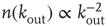, independent of the different tasks performed by the subject. We adopt this distribution for the number of presynaptic terminals of each neuron, over the range of possible values between 2 and 100. Two neurons are then connected with a distance-dependent probability, , where is their Euclidian distance [33] and a typical edge length. Once the network of output connections is established, we identify the resulting degree of in-connections, , for each neuron . An example of a small network is shown in Figure 12.1. To each synaptic connection we then assign an initial random strength , where . Moreover, synapses can have an excitatory or inhibitory character: some neurons are chosen to be inhibitory, that is, all their outgoing synapses are inhibitory, to account for a total fraction of inhibitory synapses in the network.

Figure 12.1 Three excitatory (white) neurons and one inhibitory (gray) neuron embedded in a larger network (neurons without number). Synaptic connections for the four neurons, indicated by arrows, can be excitatory (continuous lines) or inhibitory (dashed lines). The connectivity degrees are , and .

Whenever at time the value of the potential in neuron is above a certain threshold , approximately equal to for real cortical neurons, the neuron fires, that is, generates action potentials that arrive at each of the presynaptic buttons and lead to a total production of neurotransmitter proportional to , whose value can be larger than . This choice implies that the neurotransmitter production depends on the integrated stimulation received by the neuron, as it happens for real neurons where the production is controlled by the frequency of the action potential. As a consequence, the total charge that could enter into the connected neurons is proportional to . This charge is distributed among the postsynaptic neurons in proportion to the strength of the connection , which is implemented by the normalization , the total strength of all synapses outgoing from neuron to the postsynaptic neurons. The temporal evolution of the membrane voltage is therefore

12.1

where is the in-degree of neuron . This factor implies that the received charge is distributed over the surface of the soma of the postsynaptic neuron, which is proportional to the number of in-going terminals . Moreover, this normalization preserves the controlled functioning of the firing cascades in networks where highly connected neurons are present, as in scale-free networks. The plus or minus sign in Eq. (12.1) is for excitatory or inhibitory synapses, respectively. After firing, a neuron is set to zero resting membrane potential and remains in a refractory state for time steps, during which it is unable to receive or transmit any charge. We wish to stress that the unit time step in Eq. (12.1) does not correspond to a real time scale; it is simply the time unit for charge propagation from one neuron to its neighbors. The synaptic strengths have initially equal value, whereas the neuron potentials are uniformly distributed random numbers between and . Moreover, a small random fraction () of neurons are chosen to be boundary sites, with a potential fixed to 0, playing the role of sinks for the charge. An external stimulus is imposed at a random site and, if the potential reaches the firing threshold, the neuron fires and a cascade of firing neurons can evolve in the network.

12.1.1 Plastic Adaptation

As soon as a neuron is at or above the threshold at a given time , it fires according to Eq. (12.1). Then the strength of all the synapses connecting to active neurons are increased in the following way:

12.2

where is a dimensionless parameter. Conversely, the strength of all inactive synapses is reduced by the average strength increase per connection, that is,

12.3

where is the number of connections active in the previous avalanche. This normalization implements a sort of homeostatic regulation of plastic adaptation: the more active connections are strengthened, on average, the more inactive ones are weakened. The adaptation of synaptic strength is therefore tuned by a single parameter, , which represents the ensemble of all possible physiological factors influencing synaptic plasticity. The quantity depends on and on the response of the network to a given stimulus. In this way, our neuronal network “memorizes” the most used paths of discharge by increasing their synaptic strengths, whereas less used synapses atrophy. Once the strength of a synaptic connection is below an assigned small value , we remove it, that is, set it equal to 0, which corresponds to what is known as synaptic pruning. These mechanisms correspond to a Hebbian form of activity-dependent plasticity, where the conjunction of activity at the presynaptic and postsynaptic neuron modulates the efficiency of the synapse [29]. To ensure the stable functioning of neural circuits, both strengthening and weakening of Hebbian synapses are necessary to avoid instabilities due to positive feedback [34]. However, different from short-term plasticity, such as short-term facilitation or short-term depression, in our model the change of synaptic strength does not depend on the frequency of synapse activation [24, 35, 36]. It should be also considered that, in the living brain, many synapses exhibiting plasticity are chemical synapses with functional properties different from electrical synapses. For instance, Hebbian plasticity at excitatory synapses is classically mediated by postsynaptic calcium-dependent mechanisms [37]. In our approach, the excitability of the postsynaptic neuron is simply modulated by the value of the intracellular membrane potential of the presynaptic neuron.

12.2 Neuronal Avalanches in Spontaneous Activity

We applied the plasticity rules of Eqs. 12.2 and 12.3 during a series of stimuli to adapt the strengths of synapses. In fact, the more the system is actively strengthening the used synapses, the more the unused synapses will weaken. This plastic adaptation proceeds until only few connections are pruned in response to the stimuli. The system at this stage constitutes the first approximation to a trained brain, on which measurements are performed. These consist of a new sequence of stimuli, by increasing the intracellular membrane potential of a randomly selected neuron until it fires an action potential. We monitor the propagation of neuronal activity as a function of time.

After each stimulus, we measure the size distribution of the neuronal cascades (see Figure 12.2). The cascade size is defined as either the total number of firing neurons or the sum of their intracellular membrane potential variations during a cascade. This distribution exhibits a power law behavior, with an exponent equal to (see Figure 12.3). This power law identifies the cascading activity as neuronal avalanches. The avalanche activity is quite stable with respect to various parameters. The power law is also robust for densities of inhibitory synapses up to 10%, whereas it is lost for higher densities. Moreover, the distribution of avalanche durations, defined as the time period from the first spike to the last spike within an avalanche, also obeys a power law with an exponent close to (see Figure 12.3). Both these values show excellent agreement with experimental data [5]. Extensive simulations have verified that the critical behavior of avalanche distributions does not depend on parameter values or network properties (regular, small-world, Apollonian networks) [38]. Moreover, these scaling properties do not depend on the system size, indicating that the network is in a critical state and self-regulates by adjusting synaptic strengths, thereby producing the observed scale-invariant behavior.

Figure 12.2 Two neuronal avalanches in the scale-free network. Two-hundred and fifty neurons are connected by directed bonds (direction indicated by the arrow at one edge), representing the synapses. The size of each neuron is proportional to the number of in-connections, namely the number of dendrites. The two different avalanches are characterized by black and gray colors. Neurons not involved in the avalanche propagation are shown in white.

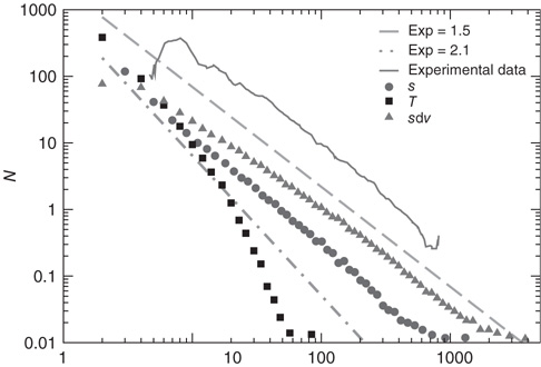
Figure 12.3 The distributions of avalanche size (circles), duration (squares), and the total potential variation during one avalanche (triangles) for 100 configurations of scale-free network with neurons (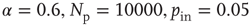). The dashed line has a slope of , whereas the dot-dashed line has a slope of . The continuous line represents the experimental distribution of avalanche sizes in rat cortex slices. Experimental data are shifted for better comparison, and no quantitative comparison is made between the size of experimental avalanches and the potential variation for numerical data.

It is interesting to notice that recently the statistics of neuronal cascades has been measured in anesthetized rats treated with a GABA inhibitor to induce epileptic behavior [39]. Under these conditions, the size distribution shows the presence of large events with a characteristic size in an almost periodic regime. This periodicity therefore induces a shoulder in the waiting time distribution, that is, the time between the beginning of two successive avalanches. Different is the case for slices of rat cortex that do not undergo any pharmacological treatment [5, 40, 41], where spontaneous activity is critical, that is, the size distribution obeys a power law over several orders of magnitude and no characteristic size or periodicity is detected.

12.2.1 Power Spectra

In order to compare with medical data, we calculate the power spectrum of the time series for neuronal activity, that is, the square of the amplitude of the Fourier transform as function of frequency. The average power spectrum (see Figure 12.4) exhibits a power law behavior with exponent over more than three orders of magnitude. This is the same value as that found generically for medical EEG power spectra [42, 43]. We also show in Figure 12.4 the magnetoelectroencephalography spectra obtained from channel 17 in the left hemisphere of a male subject resting with his eyes closed, as measured in Ref. [43], having an exponent equal to 0.795. This value is also found in the physiological signal spectra for other brain- controlled activities [44].

Figure 12.4 Power spectra for experimental data and numerical data () for the square lattice (middle line) and the Small-world lattice (bottom line, ) with rewired connections. The experimental data (top line) are from Ref. [43] and frequency is in hertz. The numerical data are averaged over 10000 stimuli in 10 different network configurations. The dashed line has a slope 0.8. Source: Novikov et al. 1997 [43]. Reproduced with permission of the American Physical Society. (We gratefully thank E. Novikov and collaborators for allowing us to use their experimental data.)

We have verified that the value of the exponent is stable against changes of the parameters , and , and also for random initial bond conductances. For , the frequency range of validity of the power law decreases by more than an order of magnitude. Figure 12.4 also shows the power spectrum for a small-world network with rewired connections and a different set of the parameters , and . The spectrum has some deviations from the power law at small frequencies but tends to the same universal scaling behavior at larger frequencies over two orders of magnitude. The same behavior is found for a larger fraction of rewired connections. We have also studied the power spectrum for a range of values of , the probability of inhibitory synapses. For a density up to 10% of inhibitory synapses, the same power law behavior is recovered within error bars. For increasing density, the scaling behavior is progressively lost and the spectrum develops a complex multipeak structure. These results suggest that the balance between excitatory and inhibitory synapses plays a crucial role for the overall behavior of the network, similar to what can occur in some severe neurological and psychiatric disorders [45, 46].

The scaling behavior of the power spectrum can be interpreted in terms of a stochastic process determined by multiple random inputs [47]. In fact, the output signal resulting from different and uncorrelated superimposed processes is characterized by a power spectrum with power law behavior and a crossover to white noise at low frequencies. The crossover frequency is related to the inverse of the longest characteristic time among the superimposed processes. The value of the scaling exponent depends on the ratio of the relative effect of a process of given frequency on the output with respect to other processes. noise corresponds to a superposition of processes of different frequencies having all the same relative effect on the output signal. In our case, the scaling exponent is smaller than unity, suggesting that processes with a high characteristic frequency are more relevant than processes with a low frequency in the superposition [47].

12.3 Learning

Next we study the learning performance of this neuronal network when it is in a critical state [48]. In order to start activity, we identify the input neurons on which the rule to be learned is applied and the output neuron on which the response is monitored. These neurons are randomly selected under the condition that they are not located at a boundary and they are separated in the network by a distance . Here, represents the chemical distance between two neurons, namely the number of connections in the shortest path between them, which differs from the Euclidian distance. can be thought of as the number of hidden layers in a perceptron. We test the ability of the network to learn different rules: AND, OR, XOR, and a random rule RAN that associates to all possible combinations of binary states at three inputs a random binary output. More precisely, the AND, OR and XOR rules are made of three input–output relations, whereas the RAN rule with three input sites implies a sequence of seven input–output relations. A single learning step requires the application of the entire sequence of states at the input neurons and then monitoring the state of the output neuron. For each rule, the binary value 1 is identified by the firing of the output neuron, that is, when the intracellular membrane potential of the output neuron reaches a value greater than or equal to at some time during the activity. Conversely, the binary state 0 at the output neuron corresponds to the state of a neuron that has been depolarized by excitatory input but failed to reach the firing threshold of the membrane potential during the entire avalanche. Once the input sites are stimulated, their activity may bring to threshold other neurons and therefore lead to avalanches of firings. We impose no restriction on the number of firing neurons, and let the avalanche evolve to its end according to Eq. (12.1). If, at the end of the avalanche, the activity did not reach the output neuron, we consider that the state of the system was unable to respond to the given stimulus and, as a consequence, to learn. We therefore increase uniformly the intracellular membrane potential of all neurons by a small quantity, , until the activity in the network has reached the output neuron, after which we compare the state of the output neuron with the desired output.

Plastic adaptation is applied to the system according to a nonuniform negative-feedback algorithm. That is, if the output neuron is in the correct state according to the rule, we keep the value of synaptic strengths. Conversely, if the response is incorrect, we modify the strengths of those synapses involved in the activity propagation by , where is the chemical distance of the presynaptic neuron from the output neuron. The sign of the adjustment depends on the nature of the incorrect response: if the output neuron fails to be in a firing state, we strengthen all active synapses by a small additive quantity proportional to . Conversely, synaptic strengths are weakened if the neuron fired when it was supposed to be silent. This adaptation rule thus provides feedback in response to the incorrect answer. The feedback is applied locally to the corresponding output neuron as well as propagating backward toward the input sites triggered locally at the output site. The biological realization of such a feedback mechanism can be thought of as a binary error signal that is locally applied at the output site and diffuses toward the input site.

Next, we analyze the performance of the system to learn different input–output rules. Figure 12.5 shows the fraction of configurations learning the XOR rule versus the number of learning steps for different values of the plastic adaptation strength . We notice that the larger the value of , the sooner the system starts to learn the rule; however, the final percentage of learning configurations is lower. The final rate of success increases as the strength of plastic adaptation decreases. This is due to the highly nonlinear dynamics of the model, where firing activity is an all-or-none event controlled by the threshold. The result that all rules give a higher percentage of success for weaker plastic adaptation is in agreement with recent experimental findings on visual perceptual learning, where better performances were measured when minimal changes in the functional network occurred as a result of learning [49].

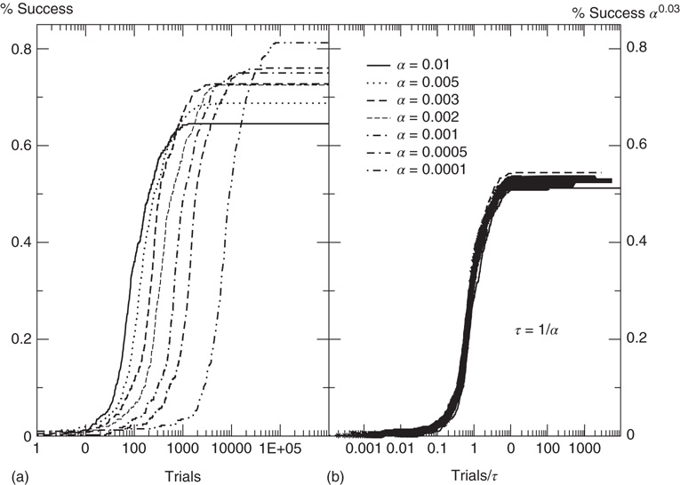
Figure 12.5 (a) Percentage of configurations learning the XOR rule as function of the number of learning steps for different plastic adaptation strengths (decreasing from bottom to top). Data are for 400 realizations of a network with neurons, and . (b) Collapse of the curves by rescaling the number of learning steps by the characteristic learning time and the percentage of success by .

We characterize the learning ability of a system for different rules by the average learning time, that is, the average number of times a rule must be applied to obtain the right answer, and the asymptotic percentage of learning configurations. This is determined as the percentage of learning configurations at the end of the teaching routine, namely after applications of the rule. The average learning time scales as for all rules, independent of the parameter values. The asymptotic percentage of success increases by decreasing as a very slow power law, , where the exponent is the average value over different rules. We check this scaling behavior by appropriately rescaling the axes in Figure 12.5. The curves corresponding to different values indeed all collapse onto a unique scaling function. Similar collapse is observed for the OR, AND, and RAN rules and for different parameters and . The dynamics of the learning process shows therefore universal properties, independent of the details of the system or the specific task assigned.

Finally, we explicitly analyze the dependence of the learning performance and its scaling behavior for different model parameters. The learning behavior is sensitive to the number of neurons involved in the propagation of the signal, and therefore depends on the distance between the input and output neurons and the level of connectivity in the system. We investigate the effect of the parameters and on the performance of the system. Systems with larger have a larger average number of synapses per neuron, producing a more branched network. The presence of several alternative paths facilitates information transmission from the inputs to the output site. However, the participation of more branched synaptic paths in the learning process may delay the time the system first gives the right answer. As expected, the performance of the system improves as the minimum out-connectivity degree increases, with the asymptotic percentage of success scaling as . On the other hand, also the chemical distance between the input and output sites plays a very important role, as the number of hidden layers in a perceptron. Indeed, as becomes larger, the length of each branch in a path involved in the learning process increases. As a consequence, the system needs a higher number of tests to first give the right answer, and a lower fraction of configurations learns the rule after the same number of steps. The percentage of learning configurations, as expected, decreases as , and similar behavior is detected for all rules. As the system size increases, the number of highly connected neurons becomes larger. A well-connected system provides better performances, therefore we could expect that the size dependence reflects the same effect. The learning performance indeed improves with the system size, since, for the same out degree distribution, the overall level of connectivity improves for larger systems.

12.4 Temporal Organization of Neuronal Avalanches

Here we focus on the overall temporal organization of neuronal avalanches both in organotypic cultures and neuronal network simulations. Each avalanche is characterized by its size , and its start and end times, and , respectively. The properties of temporal occurrence are analyzed by evaluating the distribution of waiting times . This is a fundamental property of stochastic processes, widely investigated for natural phenomena [50] and used to discriminate between a simple Poisson process and a correlated stochastic process. Indeed, in the first case the distribution is an exponential, whereas it exhibits a more complex behavior with power law regime if long-range correlations are present. For a wide variety of phenomena, for example, earthquakes, solar flares, rock fracture, and so on, this distribution always shows a monotonic behavior. In some of the chapters of this book and in an article by Ribeiro et al. [51], this distribution has been analyzed for freely behaving and anesthetized rats. The distributions show consistently a decreasing behavior. Universal scaling features are observed when waiting times are rescaled by the average occurrence rate for freely behaving rats, whereas curves for anesthetized rats do not collapse onto a unique function.

In Figure 12.6, we show the waiting time distribution for different cultures of rat cortex slices [41]. The curves exhibit a complex non-monotonic behavior with common features: an initial power law regime and a local minimum, followed by a more or less pronounced maximum. This behavior is not usually observed in natural phenomena and suggests that the timing of avalanches in organotypic cultures is not governed by a pure Poisson process. In order to investigate the origin of this behavior, we simulate avalanche activity by our model, considering that the system slowly alternates between upstates and downstates [41]. The basic idea is that, after a large avalanche, activated neurons become hyperpolarized and the system goes into a downstate where the neuronal stimulation has a small random amplitude. Conversely, after a small avalanche, active neurons remain depolarized and the system is in an upstate, where stimulation depends on the previous avalanche activity. In order to implement these mechanisms in the numerical procedure, we fix a threshold value, , for the avalanche size measured in terms of the sum of depolarizations of all active neurons, . More precisely, if the last avalanche is larger than a threshold, , the system transitions into a downstate and neurons that were active in the last avalanche become hyperpolarized proportional to their previous activity: that is, we reset

12.4

where . This rule introduces a short-range memory at the level of a single neuron and models the local inhibition experienced by a neuron, due to spike adaptation, adenosine accumulation, synaptic vesicle depletion, and so on. Conversely, if the avalanche just ended had a size , the system either will remain in an upstate or will transition into an upstate. All neurons that fired in the previous avalanche are set to the depolarized value

12.5

The neuron's intracellular potential depends on the response of the whole network via , in agreement with experimental measurements that the neuronal membrane potential remains close to the firing threshold during an upstate. controls the extension of the upstate and therefore the level of excitability of the system. The high activity in the upstate must be sustained by collective effects in the network; otherwise, the depolarized potentials would soon decay to 0, and therefore the random stimulation in the upstate has an amplitude that depends on past activity. Eqs (12.4) and (12.5) represent the simplest implementation of the neuron's upstate and downstate. Each equation depends on a single parameter, and , which ntroduce a memory effect at the level of single neuron activity and the entire system, respectively. In order to reproduce the behavior observed experimentally, the parameters and are controlled separately. However, our simulations show that the ratio is the only relevant quantity controlling the temporal organization of avalanches.

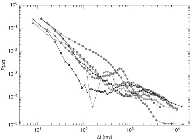
Figure 12.6 The distribution of waiting times for seven different slices of rat cortex exhibiting a non-monotonic behavior, undetected in any other stochastic process. All curves show an initial power law regime between 10 and ∼200 ms, characterized by exponent values between 2 and 2.3. For Δt > 200 ms curves can become quite different, with the common characteristics of a local minimum located at s, followed by a more or less pronounced maximum at 1–2s.

Following the above procedure, the system indeed transitions between upstates and downstates, though with different temporal durations (see Figure 12.7). The distribution of upstate durations is consistent with an exponential decay, in agreement with previous numerical results [23]. Conversely, the downstates exhibit a sharply peaked distribution with a most probable value at about 200 numerical time units. Avalanches are characterized by power law distributions for the size and the temporal duration with exponents, in good agreement with experimental results.

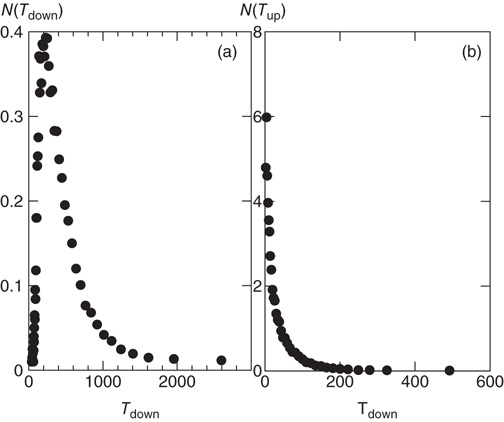
Figure 12.7 Distribution of durations of downstates (a) and upstates (b) for 100 configurations of a network of neurons with , and . Data are averaged over the number of configurations.

Next we measure the waiting time distribution between successive avalanches. In the analysis of the temporal signal, we consider avalanches involving at least two neurons, whereas single spikes are considered background noise. We measure the waiting time as the time delay between the end of an avalanche and the beginning of the next one. We notice that long waiting times generally occur after large avalanches, corresponding to downstates, whereas short ones are detected during upstates (see Figure 12.8). The scatter plot of the waiting time as a function of the previous avalanche shows that experimental data are quite scattered. In order to evidence a scaling behavior, we evaluate the expectation value of the waiting time as function of the cumulated activity over a temporal bin. These data exhibit a scaling behavior that is fully reproduced by numerical data. The good agreement between experimental and numerical results confirms the validity of our approach.

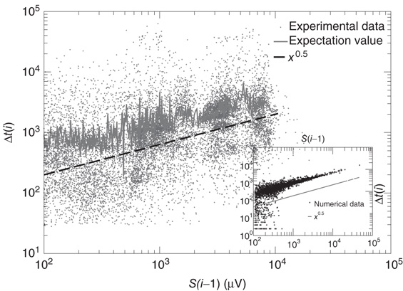
Figure 12.8 Main panel: Scatter plot of waiting time versus previous avalanche size for 15 slices of rat cortex (symbols). Expectation value of waiting time as function of the cumulated previous avalanche activity over a temporal window of 50 ms (continuous line). Data indicate that the waiting time increases with preceding avalanche activity, in line with our model assumption. Inset: Same quantity evaluated for numerical data.

The numerical waiting time distributions (see Figure 12.9) exhibit the non-monotonic behavior of the experimental curves, where the position of the minimum is controlled by the value of , and the power law regime scales with the same exponent as the experimental data. The agreement between the numerical and the experimental distributions is confirmed by the Kolmogorov–Smirnov test at the significance level. Both distributions pass the statistical test with (a) and (b). The different contribution from the two states is reflected in the activity temporal scale (inset of Figure 12.9). The upstate generates strongly clustered avalanches, yielding the power law regime of the waiting time distribution, whose extension depends on . Large between avalanches generated in the upstate are observed with a very small probability, which increases with decreasing . Conversely, the waiting time distribution evaluated in the downstate has a bell-shaped behavior centered at large waiting times which depends on , that is, for a larger disfacilitation of the network, the probability to observe intermediate waiting times decreases in favor of long . The presence of the minimum and the height of the relative maximum are sample dependent (Figure 12.7) and for each sample, simulations are able to reproduce the different behaviors by choosing the appropriate parameter values. However, the agreement between numerical and experimental data depends uniquely on the ratio , expressing the subtle balance between excitation and inhibition. For different samples, optimal agreement is realized for the same value of the ratio . For instance, enhancing the excitatory mechanism, by increasing the threshold value , clearly produces a major shift in the data [41]. Increasing the inhibitory mechanism, by tuning the hyperpolarization constant parameter , generates the opposite effect, recovering the good agreement with experimental data. It is interesting to note that the avalanche size and duration distributions exhibit the experimental scaling behavior for the set of parameters expressing the balance between the excitatory and inhibitory components.

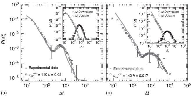
Figure 12.9 Waiting time distributions measured experimentally compared with the average numerical distributions for 100 networks with neurons. (a) Numerical curve ( and ). (b) Numerical curve ( and ). In the inset, the numerical waiting time distributions evaluated separately in the up- and down-states for the numerical statistical error bars not shown are comparable to the symbol size.

The abrupt transition between the upstate and the downstate, controlled by a threshold mechanism, produces the minimum observed experimentally. However, this mechanism alone is not sufficient to reproduce the non-monotonic behavior. Indeed, simulations of upstates and downstates only in terms of different drives, without the dependence of the single neuron state on upstate and downstates, provide a monotonic behavior [41]. The initial power law regime is followed by a plateau and a final exponential decay. The power law regime is still observed in this case, since this is mainly controlled by the drive in the upstate which introduces correlations between successive avalanches. Therefore, the introduction of inhibitory mechanisms following activity, that is, the hyperpolarizing currents in the downstate and the neuron disfacilitation, are crucial ingredients to fully reproduce the dynamics of the transition between the different activity states.

12.5 Conclusions

Several experimental evidences suggest that the brain behaves as a system acting at a critical point. This statement implies that the collective behavior of the network is more complex than the functioning of the single components. Moreover, the emergence of self-organized neuronal activity, with the absence of a characteristic scale in the response, unveils similarities with other natural phenomena exhibiting scale-free behavior, such as earthquakes or solar flares. For a wide class of these phenomena, SOC has indeed become a successful interpretive scheme. However, it is important to stress that the observation of a scale-free response is not a sufficient indication for temporal correlations among events. For instance, the waiting time distribution for the original sand pile model is a simple exponential [2] because avalanches are temporally uncorrelated. Several natural stochastic phenomena, characterized by temporal correlations and clustering, provide similar nonexponential distributions, all with a monotonic functional behavior.

Our model inspired by SOC is able to capture the scaling behavior of avalanches in spontaneous activity and to reproduce the underlying power law behavior measured by EEG in human patients. Besides reproducing neuronal activity, the network is able to learn Boolean rules via plastic modification of synaptic strengths. The implemented learning dynamics is a cooperative mechanism where all neurons contribute to select the right answer and negative feedback is provided in a nonuniform way. Despite the complexity of the model and the high number of degrees of freedom involved at each step of the iteration, the system can learn successfully even complex rules. In fact, since the system acts in a critical state, the response to a given input can be highly flexible, adapting more easily to different inputs. The analysis of the dependence of the performance of the system on the average connectivity confirms that learning is a truly collective process, where a high number of neurons may be involved and the system learns more efficiently if more branched paths are possible. The role of the plastic adaptation strength, considered as a constant parameter in most studies, provides a striking new result: the neuronal network has a “universal” learning dynamics, and even complex rules can be learned provided that the plastic adaptation is sufficiently slow.

Moreover, the temporal organization of avalanches exhibits a complex non-monotonic behavior of the waiting time distribution. Avalanches are temporally correlated in the upstate, whereas downstates are long-term recovery periods where memory of the past activity is erased. The model suggests that the crucial feature of this temporal evolution is the different single neuron behavior in the two phases. This result provides new insights into the mechanisms necessary to introduce complex temporal correlations within the framework of SOC. The good agreement with experimental data indicates that the transition from an upstate to a downstate has a high degree of synchronization. Moreover, it confirms that alternation between up- and downstates is the expression of a homeostatic regulation which, during periods of high activity, is activated to control the excitability of the system, driving it into the downstate, and avoiding pathological behavior. Network mechanisms in the upstate, where neurons mutually sustain the activity, act as a form of short-term memory. This is the crucial effect giving rise to the initial power law regime in the waiting time distribution, which is a clear sign of temporal correlations between avalanches occurring close in time in the upstate. Conversely, in the downstate, the system slowly goes back to the active state, with no memory of past activity.

These collective effects must be supported by the single neuron behavior, which toggles between two preferential states, a depolarized one in the upstate and a hyperpolarized one in the downstate. The model suggests that the depolarized neuron state is a network effect: the avalanche activity itself determines how close to the firing threshold a neuron stays in the upstate. Conversely, the hyperpolarized state is a form of temporal auto-correlation in the neuron state: the higher the neuron response during the previous avalanche, the lower is its membrane potential. The hyperpolarizing currents act as a form of memory of past activity for the single neuron. The critical state of the system is therefore the one that realizes the correct balance between excitation and inhibition via self-regulating mechanisms. This balance ensures the scale-free behavior of the avalanche activity and bursts of correlated avalanches in the upstate.

References

1. 1. Bak, P. (1996) How Nature Works: The Science of Self-Organized Criticality, Springer, New York.
2. 2. Jensen, H.J. (1998) Self-Organized Criticality: Emergent Complex Behavior in Physical and Biological Systems, Cambridge University Press, New York.
3. 3. Maslov, S., Paczuski, M., and Bak, P. (1994) Avalanches and 1/f noise in evolution and growth models. Phys. Rev. Lett., 73 (16), 2162–2165.
4. 4. Davidsen, J. and Paczuski, M. (2002) 1/f{} noise from correlations between avalanches in self-organized criticality. Phys. Rev. E, 66 (5), 050 101.
5. 5. Beggs, J.M. and Plenz, D. (2003) Neuronal avalanches in neocortical circuits. J. Neurosci., 23 (35), 11 167.
6. 6. Beggs, J. and Plenz, D. (2004) Neuronal avalanches are diverse and precise activity patterns that are stable for many hours in cortical slice cultures. J. Neurosci., 24 (22), 5216–5229.
7. 7. Gireesh, E.D. and Plenz, D. (2008) Neuronal avalanches organize as nested theta-and beta/gamma-oscillations during development of cortical layer 2/3. Proc. Natl. Acad. Sci. U.S.A., 105 (21), 7576.
8. 8. Petermann, T., Thiagarajan, T.C., Lebedev, M.A., Nicolelis, M.A.L., Chialvo, D.R., and Plenz, D. (2009) Spontaneous cortical activity in awake monkeys composed of neuronal avalanches. Proc. Natl. Acad. Sci. U.S.A., 106 (37), 15 921.
9. 9. Mazzoni, A., Broccard, F., Garcia-Perez, E., Bonifazi, P., Ruaro, M., and Torre, V. (2007a) On the dynamics of the spontaneous activity in neuronal networks. PLoS One, 2 (5), e439.
10. 10. Pasquale, V., Massobrio, P., Bologna, L., Chiappalone, M., and Martinoia, S. (2008) Self-organization and neuronal avalanches in networks of dissociated cortical neurons. Neuroscience, 153 (4), 1354–1369.
11. 11. Bak, P. and Tang, C. (1989) Earthquakes as a self-organized critical phenomenon. J. Geophys. Res., 94 (B11), 15 635–15.
12. 12. Sornette, A. and Sornette, D. (1989) Self-organized criticality and earthquakes. EPL Europhys. Lett., 9, 197.
13. 13. Bak, P. and Sneppen, K. (1993) Punctuated equilibrium and criticality in a simple model of evolution. Phys. Rev. Lett., 71 (24), 4083–4086.
14. 14. Lu, E. and Hamilton, R. (1991) Avalanches and the distribution of solar flares. Astrophys. J., 380, L89–L92.
15. 15. Politzer, P. (2000) Observation of avalanchelike phenomena in a magnetically confined plasma. Phys. Rev. Lett., 84 (6), 1192–1195.
16. 16. Faillettaz, J., Louchet, F., and Grasso, J. (2004) Two-threshold model for scaling laws of noninteracting snow avalanches. Phys. Rev. Lett., 93 (20), 208 001.
17. 17. Peters, O., Hertlein, C., and Christensen, K. (2002) A complexity view of rainfall. Phys. Rev. Lett., 88 (1), 18 701.
18. 18. Staley, K.J., Longacher, M., Bains, J.S., and Yee, A. (1998) Presynaptic modulation of ca3 network activity. Nat. Neurosci., 1, 201–209.
19. 19. Thompson, S., Haas, H., and Gähwiler, B. (1992) Comparison of the actions of adenosine at pre-and postsynaptic receptors in the rat hippocampus in vitro. J. Physiol., 451 (1), 347–363.
20. 20. Maeda, E., Robinson, H., and Kawana, A. (1995) The mechanisms of generation and propagation of synchronized bursting in developing networks of cortical neurons. J. Neurosci., 15 (10), 6834–6845.
21. 21. Sanchez-Vives, M., Nowak, L., and McCormick, D. (2000) Cellular mechanisms of long-lasting adaptation in visual cortical neurons in vitro. J. Neurosci., 20 (11), 4286–4299.
22. 22. Timofeev, I., Grenier, F., and Steriade, M. (2001) Disfacilitation and active inhibition in the neocortex during the natural sleep-wake cycle: an intracellular study. Proc. Natl. Acad. Sci. U.S.A., 98 (4), 1924.
23. 23. Millman, D., Mihalas, S., Kirkwood, A., and Niebur, E. (2010) Self-organized criticality occurs in non-conservative neuronal networks during Up states. Nat. Phys., 6 (10), 801–805, PMCID: PMC3145974.
24. 24. Albright, T.D., Jessell, T.M., Kandel, E.R., and Posner, M. (2000) Neural science: a century of progress and the mysteries that remain. Neuron, 59, S1–55.
25. 25. Hensch, T. (2004) Critical period regulation. Annu. Rev. Neurosci., 27, 549–579.
26. 26. Abbott, L. and Nelson, S. et al. (2000) Synaptic plasticity: taming the beast. Nat. Neurosci., 3, 1178–1183.
27. 27. Hebb, D. (1949) The Organization of Behavior, John Wiley & Sons, Inc., New York.
28. 28. Tsien, J. (2000) Linking hebb's coincidence-detection to memory formation. Curr. Opin. Neurobiol., 10 (2), 266–273.
29. 29. Cooper, S. (2005) Donald O. Hebb's synapse and learning rule: a history and commentary. Neurosci. Biobehav. Rev., 28 (8), 851–874.
30. 30. de Arcangelis, L., Perrone-Capano, C., and Herrmann, H. (2006b) Self-organized criticality model for brain plasticity. Phys. Rev. Lett., 96 (2), 28 107.
31. 31. Pellegrini, G.L., de Arcangelis, L., Herrmann, H., and Perrone-Capano, C. (2007) Activity-dependent neural network model on scale-free networks. Phys. Rev. E, 76 (1), 016 107.
32. 32. Eguiluz, V., Chialvo, D., Cecchi, G., Baliki, M., and Apkarian, A. (2005) Scale-free brain functional networks. Phys. Rev. Lett., 94 (1), 18 102.
33. 33. Roerig, B. and Chen, B. (2002) Relationships of local inhibitory and excitatory circuits to orientation preference maps in ferret visual cortex. Cereb. Cortex, 12 (2), 187–198.
34. 34. Desai, N. (2003) Homeostatic plasticity in the cns: synaptic and intrinsic forms. J. Physiol.-Paris, 97 (4-6), 391–402.
35. 35. Paulsen, O. and Sejnowski, T. (2000) Natural patterns of activity and long-term synaptic plasticity. Curr. Opin. Neurobiol., 10 (2), 172–180.
36. 36. Braunewell, K. and Manahan-Vaughan, D. (2001) Long-term depression: a cellular basis for learning? Rev. Neurosci., 12 (2), 121.
37. 37. Bi, G. and Poo, M. (2001) Synaptic modification by correlated activity: Hebb's postulate revisited. Annu. Rev. Neurosci., 24 (1), 139–166.
38. 38. de Arcangelis, L. and Herrmann, H. (2012) Activity-dependent neuronal model on complex networks. Front. Physiol., 3, 62.
39. 39. Osorio, I., Frei, M., Sornette, D., Milton, J., and Lai, Y. (2010) Epileptic seizures: quakes of the brain?. Phys. Rev. E, 82 (2), 021 919.
40. 40. Stewart, C. and Plenz, D. (2006) Inverted-u profile of dopamine–nmda-mediated spontaneous avalanche recurrence in superficial layers of rat prefrontal cortex. J. Neurosci., 26 (31), 8148–8159.
41. 41. Lombardi, F., Herrmann, H., Perrone-Capano, C., Plenz, D., and de Arcangelis, L. (2012) Balance between excitation and inhibition controls the temporal organization of neuronal avalanches. Phys. Rev. Lett., 108 (22), 228 703.
42. 42. Freeman, W., Rogers, L., Holmes, M., and Silbergeld, D. (2000) Spatial spectral analysis of human electrocorticograms including the alpha and gamma bands. J. Neurosci. Methods, 95 (2), 111–121.
43. 43. Novikov, E., Novikov, A., Shannahoff-Khalsa, D., Schwartz, B., and Wright, J. (1997) Scale-similar activity in the brain. Phys. Rev. E, 56 (3), 2387–2389.
44. 44. Hausdorff, J., Ashkenazy, Y., Peng, C., Ivanov, P., Stanley, H., and Goldberger, A. (2001) When human walking becomes random walking: fractal analysis and modeling of gait rhythm fluctuations. Physica A, 302 (1), 138–147.
45. 45. Rubenstein, J. and Merzenich, M. (2003) Model of autism: increased ratio of excitation/inhibition in key neural systems. Genes, Brain Behav., 2 (5), 255–267.
46. 46. Powell, E., Campbell, D., Stanwood, G., Davis, C., Noebels, J., and Levitt, P. (2003) Genetic disruption of cortical interneuron development causes region-and gaba cell type-specific deficits, epilepsy, and behavioral dysfunction. J. Neurosci., 23 (2), 622–631.
47. 47. Hausdorff, J. and Peng, C. (1996) Multiscaled randomness: a possible source of 1/f noise in biology. Phys. Rev. E, 54 (2), 2154.
48. 48. de Arcangelis, L. and Herrmann, H. (2010) Learning as a phenomenon occurring in a critical state. Proc. Natl. Acad. Sci. U.S.A., 107 (9), 3977–3981.
49. 49. Lewis, C., Baldassarre, A., Committeri, G., Romani, G., and Corbetta, M. (2009) Learning sculpts the spontaneous activity of the resting human brain. Proc. Natl. Acad. Sci. U.S.A., 106 (41), 17–558–17–563.
50. 50. de Arcangelis, L., Godano, C., Lippiello, E., and Nicodemi, M. (2006a) Universality in solar flare and earthquake occurrence. Phys. Rev. Lett., 96 (5), 51 102.
51. 51. Ribeiro, T., Copelli, M., Caixeta, F., Belchior, H., Chialvo, D., Nicolelis, M., and Ribeiro, S. (2010) Spike avalanches exhibit universal dynamics across the sleep-wake cycle. PloS One, 5 (11), e14 129.