13
The Neuronal Network Oscillation as a Critical Phenomenon
13.1 Introduction
When investigating nature we often discard the observed variation and describe its properties in terms of an average, such as the mean or median [1]. For some objects or processes, however, the average value is a poor description, because they do not have a typical or “characteristic” scale. Such systems are broadly referred to as scale-free [2]. There is growing evidence that physiological processes can exhibit fluctuations without characteristic scales and that this scale-free dynamics is important for their function [2–8]. Heuristically, one may reason that scale-free dynamics implies a wide range of functional states, which is characteristic for physiological systems in general and neuronal networks in particular.
Synchronous brain activity is thought to be crucial for neural integration, cognition, and behavior [9] [10]. The multiscale properties of synchronous cell assemblies, however, remain poorly understood. While probing activity at different scales, several investigators have begun to consider self-organized criticality (SOC) as an overriding neuronal organizing principle [7] [11–22]. The SOC theory holds that slowly driven, interaction-dominated threshold systems will be attracted to a critical point, with the system balanced between order and disorder [3] [23, 24].
This critical state is characterized by scale-free probability distributions. In cortical slices, “neuronal avalanches” of local field potential activity are governed by a power-law (i.e., scale-free) distribution of event sizes with an exponent of −1.5, as expected for a critical branching process [12]. Similar results have also been found in vivo [19]. This finding inspired the development of computational models that were capable of producing power-law-distributed neuronal avalanches through a process of self-organization, thereby providing theoretical support for SOC in neuronal systems [15] [21, 22]. Models have shown that networks in a critical state display differing responses to the widest input range [14], with the largest repertoire of metastable patterns [13], and maximal information and transmission capacity [25] [26]. Scale-free dynamics have been observed on many levels of neuronal organization. Power-law scaling is, for example, found in the decay of temporal correlations in behavioral performance [1], and in the phase-locking intervals between brain regions [27] [28].
Interestingly, ongoing oscillations measured with electroencephalography (EEG) or magnetoencephalography (MEG) exhibit power-law-scaled temporal (auto-)correlations in their amplitude modulation, also known as long-range temporal correlations (LRTCs) [11] [29]. Given that neuronal avalanches and oscillations depend on balanced excitation and inhibition [12] [26, 30], it is plausible that their scale-free dynamics are related. In this chapter, we explain the methods used for studying scale-free dynamics of neuronal oscillations and provide examples of these analyses applied to the amplitude dynamics in health and disease. Further, we describe the concept of multilevel criticality as a state where scale-free behavior emerges jointly on different levels of network dynamics: the short-time-scale spreading of activity in the form of avalanches, with an upper bound at the characteristic timescale of the dominant oscillation, and the long-time-scale modulation of the oscillatory amplitude.
13.2 Properties of Scale-Free Time Series
Detrended fluctuation analysis (DFA) is widely used for quantifying LRTCs and scaling behavior in neuronal time series, because it provides a more reliable estimate of scaling exponents than the autocorrelation function or the power-spectrum density [31–33]. The signal-processing steps in DFA have often been reported [11] [34]; however, the concepts of self-affinity and stationarity are fundamental to understanding why DFA provides a measure of correlations over time and, therefore, we shall first explain these.
13.2.1 Self-Affinity
Self-affinity is a property of fractal time series [35] [36]. It is a special case of self-similarity, according to which a small part of a fractal structure is similar to the whole structure. When this small part is an exact replica of the whole then the fractal is exact, which is the case for purely mathematical and geometrical fractals (e.g., the van Koch curve and the Mandelbrot tree) [37]. When the self-similarity is expressed in terms of statistical properties (e.g., the mean and standard deviation for a portion of a fractal are scaled versions of the mean and standard deviation of the whole), then the fractal is a statistical fractal. While the self-similarity property is isotropic and applies along all the dimensions of a fractal object, self-affinity describes anisotropic scaling, where statistical properties of the fractal scale differently along different dimensions. In the case of a time series, the time dimension is rescaled.
Nature hosts some intriguing examples of self-similar structures, such as the Roman cauliflower (Romanesco broccoli), in which almost exact copies of the entire flower may be recognized on multiple smaller scales (Figure 13.1A). Physiological time series may exhibit statistical self-affine properties [38] [39]. Self-affine processes and self-similar structures have in common that the statistical distribution of the measured quantity follows a power-law function, which is the only mathematical function without a characteristic scale. Self-affine and self-similar phenomena are therefore called scale-free.
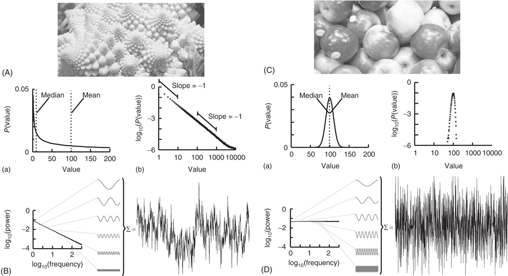
Figure 13.1 The Roman cauliflower is a striking example of self-similarity in nature. (A) The cauliflower is composed of flowers that are similar to the entire cauliflower. These smaller flowers, in turn, are composed of flowers that are similar to the entire cauliflower or the intermediate flowers. The self-similarity is apparent on at least four levels of magnification, thereby illustrating the scale-free property that is a consequence of self-similarity. (a) A hypothetical distribution of the likelihood of flowers on a cauliflower having a certain size. This property is captured by the power-law function. The mean or median of a power law, however, provides a poor representation of the scale-free distribution (and in a mathematical sense is not defined). (b) The power-law function makes a straight line in double-logarithmic coordinates. The slope of this line is the exponent of the power law, which captures an important property of scale-free systems, namely, the relationship between the size of objects or fluctuations on different scales, that is, the slope between 1 and 10 is the same as the slope between 100 and 1000 (both −1). (B) Time signals can also be viewed as self-affine as they can be transformed into a set of sine waves of different frequencies. In a 1/f signal, the lower frequency objects have larger amplitude than the higher frequency objects, which we can compare with there being fewer large cauliflowers than there are small cauliflowers. (C) As the size of apples shows smaller variation, they are well described by taking an average value such as the mean or median. (a) Hypothetical distribution showing the likelihood of apples having a certain size. Both the mean and median are good statistics to convey the size of the apples. (b) Plotting the normal distribution on double-logarithmic coordinates has little effect on the appearance of the distribution, which still shows a characteristic scale. (D) A white-noise signal is also self-affine, but now the lower frequency objects have the same amplitude as the higher frequency objects, meaning that only the high-frequency fluctuations are visible in the signal.
Considering again the example of the Romanesco broccoli, we can say that it is a “scale-free” structure, because there is no typical size of flower on the cauliflower, with the frequency of a certain size of flower being inversely proportional to its size. A scale-free time series will in a similar manner be composed of sine waves with amplitudes inversely proportional to their frequency (Figure 13.1B), seen as a straight line when the power spectrum is plotted on a double-logarithmic axis. This is in contrast to the wide variety of objects that have a typical scale, for example, the size of the apples on a tree (Figure 13.1C). None of them will be very small or very large; rather, they will form a Gaussian distribution centered on some characteristic size, which is well represented by the mean of the distribution. Qualitatively, the characteristic scale is present at the expense of rich variability. Similarly, a time series in which all frequencies are represented with the same characteristic amplitude will lack the rich variability of the scale-free time series and is referred to as white noise (Figure 13.1D). Phenomena with characteristic scales are well defined by their mean and standard deviation (Figure 13.1C,D), whereas scale-free phenomena are better described by the exponent of a power-law function, because it captures the relationship between objects or fluctuations on different scales (Figure 13.1A,B).
Let us now introduce the mathematical definitions:
A nonstationary stochastic process is said to be self-affine in a statistical sense, if a rescaled version of a small part of its time series has the same statistical distribution as the larger part. For practical purposes, it is sufficient to assess the standard deviation. Thus, the process,  , is self-affine if for all windows of length t [40]:
where:
- “
 ” and “
 ” are values of a process at time windows of length
  and
and  , respectively
 - “L”: window-length factor
- “H”: Hurst exponent, dimensionless estimator of self-affinity
- “≡”: the standard deviation on both sides of the equation are identical.
To illustrate the implications of this definition for the property of a self-affine process, we consider a Hurst exponent of 0.75 and derive the standard deviation for two and three times the length of the timescale. To double the timescale, we set L = 2;
Therefore, the standard deviation of a signal twice the length of  is
is  times larger than that of the original signal
  .
.
Tripling the window size with L = 3 gives:
The standard deviation increases by a factor of  . In other words, with a Hurst exponent H = 0.75, the standard deviation grows with increasing window size according to the power law,
  , as indicated in Eq. (13.1). This mathematical formulation shows another property of self-affine processes, which is scale invariance: the scaling of the standard deviation is not dependent on the absolute scale. A signal exhibiting the described behavior is also said to exhibit “scale-free” fluctuations with a “power-law scaling exponent” H. H is the Hurst exponent [41] and ranges between 0 and 1. For signals with H approaching 1, the appearance is smooth, typically meaning that high values are followed by high values (or low values are followed by low values). This lack of independency over time implies that the time series is temporally correlated. In contrast, for signals with H close to 0, the appearance is rough and “hairy,” which typically means faster switching between high and low values.
The estimation of the scaling exponent is particularly interesting for neuronal oscillation dynamics, because it can reveal the presence of LRTCs in neuronal network oscillations [11]. In the following sections, we show you how.
13.2.2 Stationary and Nonstationary Processes
When performing scale-free analysis of a time series, it is essential to have a model of whether the underlying process is stationary. This is because many of the methods used on a time series to estimate H make assumptions about whether the process is stationary or not. For example, self-affinity as described only applies to nonstationary processes, because by definition the variance of a stationary process does not alter with the amount of time looked at [40].
Nevertheless, scale-free processes that are stationary also exist and can be modeled as so-called fractional Gaussian noise (fGn), whereas nonstationary processes are modeled as fractional Brownian motion (fBm). There is an important relationship, however, between these two types of processes in that, by definition, the increments of a fBm process are modeled as an fGn process with the same Hurst exponent; for more details on these models, see [38] [42]. This relationship allows us to apply the definition of self-affinity given here to a stationary fGn process, by first converting it into its nonstationary fBm equivalent as follows. Given the time series  , we define the signal profile as the cumulative sum of the signal:
where  is the mean of the time series. The subtraction of the mean eliminates the global trend of the signal. The advantage of applying scaling analysis to the signal profile instead of the signal is that it makes no a priori assumptions about the stationarity of the signal. When computing the scaling of the signal profile (as explained subsequently), the resulting scaling exponent, α, is an estimation of H. If α is between 0 and 1, then x was produced by a stationary process, which can be modeled as an fGn process with H = α. If α is between 1 and 2, then x was produced by a nonstationary process, and H = α − 1 [38].
13.2.3 Scaling of an Uncorrelated Stationary Process
We now show that the scaling of a so-called random-walk process can be used to infer whether a time series is uncorrelated. A random walk is a nonstationary probabilistic process derived from the cumulative sum of independent random variables, where each variable has equal probability to take a value of 1 or −1. Imagine a walker that at each time step can either take one step left (−1) or right (+1) with equal probabilities. The sequence of the steps representing independent random variables forms a stationary time series as it can only take two values, which do not depend on time. If we calculate the standard deviation of this time series for differently sized time windows, we will not see a scaling effect as there will always on average be an equal number of 1's and −1's. As the probability of taking either action does not depend on any previous actions, the process is said to be “memory-less.”
Now, if we compute the cumulative sum of this time series, using Eq. (13.2) to obtaining the random walk, we can calculate the distance that the walker deviates from the zero line where it started (following a given number of steps). This distance changes with the number of steps that the walker has taken. Therefore, it is possible to calculate how the standard deviation of distance from the origin (referred to as random-walk fluctuations) changes depending on the number of steps that the walker has taken.
We can calculate this by working out the relationship between the displacement,  , at time t and time t + 1. If at time t the walker is at position
  then at time t + 1 the walker will be at position
  or
or  with equal likelihood. Therefore, we can calculate the mean square displacement at time t + 1:

Let us define the starting position to be 0, that is, the mean square displacement at time 0 is

Now, we can calculate the mean square displacement after an arbitrary number of steps by applying Eq. (13.3) iteratively:
Thus, the mean square displacement after a walk of L steps is L, or equivalently, the root-mean-square displacement after L steps is the square root of L:
For a zero-mean signal,  , the root-mean-square displacement is the standard deviation. Thus, the cumulative sum of a randomly fluctuating zero-mean signal will have the standard deviation growing with window length, L, according to a power law with the exponent of 0.5. Now, recall from Eq. (13.1) that if the standard deviation of a signal scales by a factor
  according to the length of the signal, L, then the process exhibits self-affinity with Hurst exponent H. Thus, we have derived that a stationary randomly fluctuating process has a signal profile, which is self-affine with a scaling exponent α = 0.5.
13.2.4 Scaling of Correlated and Anticorrelated Signals
What happens to the self-affinity of a process when we add memory in the sense that the probability of an action depends on the previous actions that the walker has made? Different classes of processes with memory exist. Let us focus on those with positive correlations and those with anticorrelations. Anticorrelations can be seen as a stabilizing mechanism: any action the walker makes means that when taking future actions the walker will be more likely to take the opposite action (Figure 13.2A-a). This leads to smaller fluctuations on longer timescales than seen by chance (Figure 13.2B). Positive correlations have the opposite effect: Any action the walker takes makes it more likely to take that action in the future (Figure 13.2A-c). This leads to large fluctuations in the integrated signal (Figure 13.2B). We define a fluctuation function as the standard deviation of the signal profile:
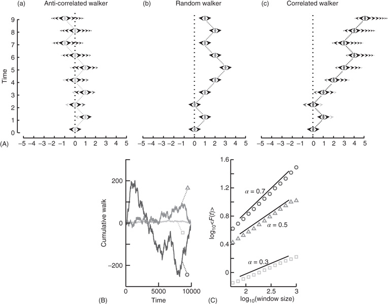
Figure 13.2 Processes with a memory produce qualitatively, and quantitatively, different fluctuations compared to a random-walk process. (A) Correlations occur when the “walker's” decision to follow a certain direction is influenced by its past actions. (a) Path of an anticorrelated walker shown over time. At each time step, the walker makes a decision based on a weighted choice between left and right. The weighted choice can be seen by the sum of the areas of the arrows pointing left and right. Each action the walker takes continues to influence future actions, with the walker being more likely to take the opposite action. This is illustrated as a gradual accumulation of arrows that refer to past actions, but also decrease in size over time, because the bias contributions of those actions decay over time. The light gray arrows show how the first action the walker takes (going right) persists over time, with the influence getting smaller as time goes on seen by the dark arrow size decreasing. (b) Path of a random walker shown over time. The random walker is not influenced by previous actions and so always has equal probability of going left or right. (c) Path of a correlated walker shown over time. Here, each action the walker takes influences future actions by making the walker more likely to take that action. The light gray shows that by taking the action of going right at time 0, the walker is more likely to go right in future time steps with the influence getting smaller as time goes on. (B) Cumulative signal for a positively correlated process (dark gray, circle) shows larger fluctuations over time than a random walker (gray, triangle). An anticorrelated signal (light gray, square) shows smaller fluctuations over time. (C) By looking at the average fluctuations for these different processes at different timescales, we can quantify this difference. A random walker shows a scaling exponent of 0.5, with the positively correlated process having a larger exponent, and the anticorrelated process having a smaller exponent. (Modified from [33].)
We note from Eq. (13.4) that this function grows as a power law with scaling exponent α = 0.5 for a stationary random signal. Using Eq. (13.5) – and as shown in Figure 13.2C – it follows that if the fluctuations scale according to time with:
- 0 < α < 0.5 then the process has a memory, and it exhibits anticorrelations (can be modeled by fGn with H = α).
- 0.5 < α < 1 then the process has a memory, and it exhibits positive correlations (can be modeled by fGn with H = α).
- α = 0.5 then the process is indistinguishable from a random process with no memory (can be modeled by fGn with H = α).
- 1 < α < 2 then the process is nonstationary (can be modeled as a fBm with H = α − 1).
For short-range correlations, the scaling exponent will deviate from 0.5 only for short window sizes, because the standard deviation of the integrated signal in long windows will be dominated by fluctuations that have no dependence on each other. Thus, it is important to report the range where the scaling is observed. We return to the practical issues of identifying the scaling range in the section on “Insights from the application of DFA to neuronal oscillations.”
13.3 The Detrended Fluctuation Analysis (DFA)
We have seen that calculating the fluctuation of signal profiles in windows of different sizes can be used to quantify the scale-free nature of time series. However, calculating the fluctuations at a certain timescale is strongly influenced by whether the signal has a steady trend on longer timescales. This trend is unlikely to be part of a process on the timescale of that window and may be removed by subtracting the linear trend in the window, and then calculating the standard deviation. This way we know that processes on scales larger than the given window size will only marginally influence the fluctuation function, Eq. (13.5).
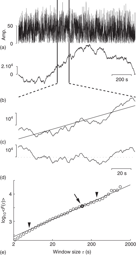
Figure 13.3 Step-wise explanation of detrended fluctuation analysis. (a) Time series with a sampling rate of 300 Hz and a duration of 1200 s. (b) Cumulative sum of signal shows large fluctuations away from the mean. (c) For each window looked at, calculate the linear trend (straight line). (d) Fluctuation is calculated on the window after removing the linear trend. (e) Plot the mean fluctuation per window size against window size on logarithmic axes. The DFA exponent is the slope of the best-fit line.
The idea to remove the linear trend was introduced by Peng et al. [43] as DFA with less strict assumptions about the stationarity of the signal than the autocorrelation function. Since then, the algorithm has been applied in more than a 1000 studies, and it is one of the most commonly used methods to quantify the scale-free nature of physiological time series and their alteration in disease [34] [44, 45]. The DFA is based on the rationale described in the sections presented so far, and can be summarized as follows:
- Compute the cumulative sum of the time series (Figure 13.3a) to create the signal profile (Figure 13.3b).
- Define a set of window sizes, T, which are equally spaced on a logarithmic scale between the lower bound of four samples [43] and the length of the signal.
- For each window length τ ∈ T
- Split the signal profile into a set (W) of separate time series of length t, which have 50% overlap.
- For each window w ∈ W
- Remove the linear trend (using a least-squares fit) from the time series (Figure 13.3c) to create wdetrend (Figure 13.3d)
- Calculate the standard deviation of the detrended signal, σ(wdetrend)
- Compute fluctuation function as the mean standard deviation of all identically sized windows:<F(t)> = mean(σ(W)
- For each window length τ ∈ T
- Plot the fluctuation function for all window sizes, T, on logarithmic axes (Figure 13.3e).
- The DFA exponent, α, is the slope of the trend line in the range of timescales of interest and can be estimated using linear regression (Figure 13.3e).
Here, we have chosen logarithmically spaced window sizes, because it gives equal weight to all timescales when we fit a line in log–log coordinates using linear regression. The lower end of the fitting range is at least four samples, because linear detrending will perform poorly with less points [43]. For the high end of the fitting range, DFA estimates for window sizes >10% of the signal length are more noisy because of a low number of windows available for averaging (i.e., less than 10 windows). Finally, the 50% overlap between windows is commonly used to increase the number of windows, which can provide a more accurate estimate of the fluctuation function especially for the long-time-scale windows.
The DFA exponent is interpreted as an estimation of the Hurst exponent, as explained with the random-walker example, that is, the time series is uncorrelated if α = 0.5. If 0.5 < α < 1, then there are positive correlations present in the time series as you are getting larger fluctuations on longer timescales than expected by chance. If α < 0.5, then the time series is anticorrelated, which means that fluctuations are smaller in larger time windows than expected by chance.
Since DFA was first introduced, several papers have validated the robust performance of DFA in relation to trends [46], nonstationarities [47], preprocessing such as artifact rejection [47], and coarse graining [48].
13.4 DFA Applied to Neuronal Oscillations
Synchronized activity between groups of neurons occurs in a range of frequencies spanning at least four orders of magnitude from 0.01 to 100 Hz [10]. The power spectral density plotted on double-logarithmic axes roughly follows a power-law distribution, but there may also be several “peaks” seen along it, corresponding to the classical frequency bands (e.g., θ, α, β, etc.). In this section, we describe how to apply DFA analysis to the amplitude modulation in these frequency bands, and show how they have been utilized in quantifying healthy and pathological conditions. We cannot apply DFA directly to the band-pass-filtered signal, because it will appear as a strongly anticorrelated signal because of the peaks and troughs averaging out when computing the cumulative sum. Instead, we focus on the amplitude envelope of oscillations.
The method consists of four steps:
- Preprocess the signals.
- Create band-pass filter for the frequency band of interest.
- Extract the amplitude envelope and perform DFA.
- Determine the temporal integration effect of the filter to choose the window sizes for calculating the DFA exponent.
13.4.1 Preprocessing of Signals
Sharp transient artifacts are common in EEG signals. These large jumps in the EEG signal on multiple channels are, for example, caused by electrode movement. Leaving these in the signal is likely to affect the DFA estimates, whereas removing them has little effect on the estimated exponent [47]. Other artifacts from, for example, eye movement, respiration, and heartbeat are also likely to disturb the estimate and are better removed. Another factor that can influence the DFA estimate is the signal-to-noise ratio (SNR) of the signal. The lower this ratio, the more biased the estimated scaling is toward an uncorrelated signal. Simulations indicated that a SNR > 2 is sufficient to accurately determine LRTC [32].
13.4.2 Filter Design
To filter the EEG/MEG data (Figure 13.4A), we use a band-pass finite-impulse-response (FIR) filter. This is used instead of an infinite impulse response (IIR) filter to avoid introducing long-range correlations in the signal before calculating the fluctuation function. The filter order for the FIR filter is recommended to be set to two cycles of the lowest frequency in order to accurately detect the oscillations while also limiting the temporal integration caused by the filter. In Figure 13.4B we can see a clear peak in the α-band frequency range (8–13 Hz) and, therefore, we would band-pass filter in this frequency range with a filter order set to two cycles of 8 Hz.
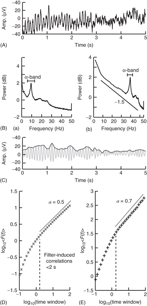
Figure 13.4 Step-wise explanation of applying DFA to neuronal oscillations. (A) EEG recording from electrode Oz shows clear oscillations during a 15 min eyes-closed rest session. Data were recorded at 250 Hz and band-passed filtered between 0.1 and 200 Hz. (B) Power spectrum (Welch method, zero padded) shown in logarithmic (a) and double-logarithmic axes (b), shows clear peak in the α band. (C) Signal in (A) filtered in the α band (8–13 Hz) using an FIR filter with an order corresponding to the length of two 8 Hz cycles (light gray). Amplitude envelope (black) calculated using the Hilbert transform. (D) DFA applied to the amplitude envelope of white-noise signal filtered using the same filter as in (C). At time windows <2 s, filter-induced correlations are visible through a bend away from the 0.5 slope. (E) DFA applied to the amplitude envelope of the α-band-filtered EEG signal shows long-range temporal correlations between 2 and 90 s with exponent α = 0.71.
13.4.3 Extract the Amplitude Envelope and Perform DFA
When applying DFA to neuronal oscillations, we are interested in how the amplitude of an oscillation changes over time. To calculate this, we extract the amplitude envelope from the filtered signal by taking the absolute value of the Hilbert transform (Figure 13.4C) [49]. The Hilbert transform is easily accessible in most programming languages (e.g., scipy.signal.Hilbert in Python (Scipy), Hilbert in Matlab). Wavelet transforms, however, have also been used to extract the amplitude envelope [11]. Once you have the amplitude envelope, you can perform DFA on it (Figure 13.4E). However, to decide which window sizes to calculate the exponent from, you first need to follow step 4.
13.4.4 Determining the Temporal Integration Effect of the Filter
Filtering introduces correlation in the signal between the neighboring samples (e.g., owing to the convolution in case of FIR filtering). Thus, including very small window sizes in the fitting range of the fluctuation function will lead to an overestimation of temporal correlations (Figure 13.4D). The effect of a specific filter on the DFA may be estimated using white-noise signals (where a DFA exponent of 0.5 is expected) [50]:
13.5 Insights from the Application of DFA to Neuronal Oscillations
The discovery of LRTCs in the amplitude envelope of ongoing oscillations was based on 20 min recordings of EEG and MEG during eyes-closed and eyes-open rest [11]. In both conditions, amplitude envelopes of α and β oscillations exhibited power-law scaling behavior on timescales of 5–300 s with DFA exponents significantly higher than for band-pass-filtered white noise. These results were further validated by showing 1/f power spectra and a power-law decay in the autocorrelation function.
The robustness of LRTC in ongoing oscillations has been confirmed in several follow-up studies, albeit often based on shorter experiments and scaling analysis in the range of about 1–25 s [29] [32, 51] [52]. The power-law scaling behavior in the θ band is reported less often [52], and, to our knowledge, LRTC in the delta band have only been investigated in subdural EEG [29]. LRTC have also not been reported often in the gamma band owing to the low SNR obtained from EEG/MEG recordings in this band. Invasive recordings in nonhuman primates, however, have reported 1/f spectra for the amplitude modulation in both low and high gamma bands [53]. Recordings from the subthalamic nucleus in Parkinson patients even show prominent LRTC in the very high-frequency gamma range (>200 Hz), especially when treated with the dopamine-precursor drug Levodopa [54].
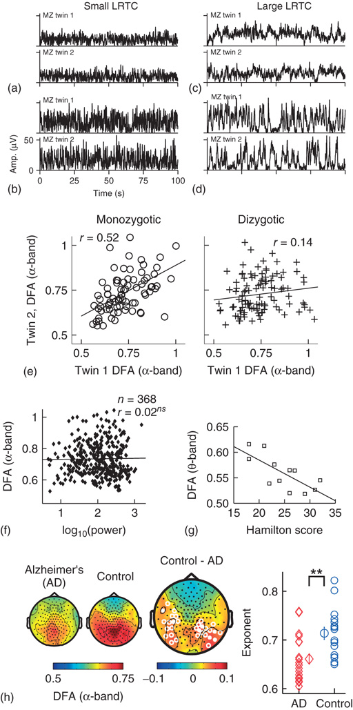
Figure 13.5 Results of applying DFA to neuronal oscillations. (a–d) Individual differences in long-range temporal correlations in α oscillations are, to a large extent, accounted for by genetic variation, which can be seen qualitatively by looking at four sets of monozygotic twins. (Figure modified from [32].) (e) The effect of genetic variation on LRTC can be quantified by the difference in correlations of DFA exponents between monozygotic and dizygotic twins. (Figure modified from [32].) (f) The DFA exponent is independent of oscillation power. Data were recorded using EEG on 368 subjects during a 3 min eyes-closed rest session. (Figure modified from [32].) (g) DFA exponents of θ oscillations in the left sensorimotor region correlate with the severity of depression based on the Hamilton score. Data recorded from 12 depressed patients with MEG, during an eyes-closed rest session of 16 minutes. (Figure modified from [55].) (h) DFA of α oscillations shows a significant decrease in the parietal area in patients with Alzheimer's disease than in controls. MEG was recorded during 4 min of eyes-closed rest and the DFA exponent estimated in the time range of 1–25 s. (Right) Individual-subject DFA exponents averaged across significant channels are shown for the patients diagnosed with early-stage Alzheimer's disease (n = 19) and the age-matched control subjects (n = 16). (Figure modified from [56].)
To gain validity for LRTC, it has been shown that LRTC have a link to the underlying genetics of the subject. This link was provided in [32] where the scaling of eyes-closed rest EEG from monozygotic and dizygotic twin subjects (n = 368) showed that ∼60% of the variance of DFA exponents in the α- and β-frequency bands is attributable to genetic factors (Figure 13.5a–e). This was an important result as it clearly showed that the nonrandom patterns of fluctuations in the ongoing oscillations are governed by low-level biological factors as opposed to uncontrolled experimental variables during the recording sessions. The finding also provides an explanation of the significant test–retest reliability of DFA exponents [50].
Several studies have reported that DFA exponents of neuronal oscillations are independent of oscillation power for a given frequency band, both when the oscillations are recorded with subdural EEG [29] and scalp EEG [32] [52] (Figure 13.5f). These results together indicate that the DFA can be used as a robust measure of oscillatory dynamics, which captures features of brain activity different from those seen in classical analysis such as power in a frequency band.
13.5.1 DFA as a Biomarker of Neurophysiological Disorder
We have so far discussed the results of applying DFA to healthy subjects; however, some of the most exciting results have come from preclinical studies, which indicate possible functional roles for LRTC. For example, a breakdown of LRTC in the amplitude fluctuations of resting-state θ oscillations detected in the left sensorimotor region was reported for patients with major depressive disorder [55]. Interestingly, the severity of depression, as measured by the Hamilton depression rating scale, inversely correlated with the DFA exponent of the patients (Figure 13.5g). Reduction in the LRTC of oscillations has also been reported in the α band in the parietal region in patients with Alzheimer's disease [56] (Figure 13.5h). Furthermore, reduction in the α and β bands in the centroparietal and frontocentral areas has also been reported for patients with schizophrenia [57].
Interestingly, it seems as though it is not only a loss of LRTC that correlates with disorders but also elevated levels of LRTC. Monto et al. [29] looked at different scales of neuronal activity by using subdural EEG to record the areas surrounding an epileptic focus in five patients during ongoing seizure-free activity. They discovered that the LRTC are abnormally strong near the seizure-onset zone. Further, it was shown that administration of the benzodiazepine lorazepam to the patients leads to decreased DFA exponents in the epileptic focus, suggesting that the pharmacological normalization of seizure activity brings with it also a normalization of LRTC. Interestingly, however, DFA exponents were observed to increase in the seizure-free surrounding areas, which may correspond to the increase in LRTC observed in vitro after application of Zolpidem, which is also a GABAergic modulator [58].
Overall, these studies seem to indicate that there is an optimal level of temporal structure of oscillations and any deviation from this can result in a significant loss of function. Importantly, early studies have estimated the DFA exponent from the scaling of the fluctuation function across almost two orders of magnitude in time [11] [29, 59] [60], whereas most reports have used one decade of fitting range and found the DFA a very useful biomarker to study neuronal dynamics in health and disease.
13.6 Scaling Behavior of Oscillations: a Sign of Criticality?
The LRTCs in neuronal oscillations reviewed in the previous sections have often been suggested to reflect neuronal networks operating in a critical state. Critical dynamics of oscillatory networks, however, would ideally be accompanied by scale-free spatial distributions of neuronal activation patterns. To investigate this, Poil et al. [61] have modeled a generic network of excitatory and inhibitory neurons in which the local connectivities could be varied systematically.
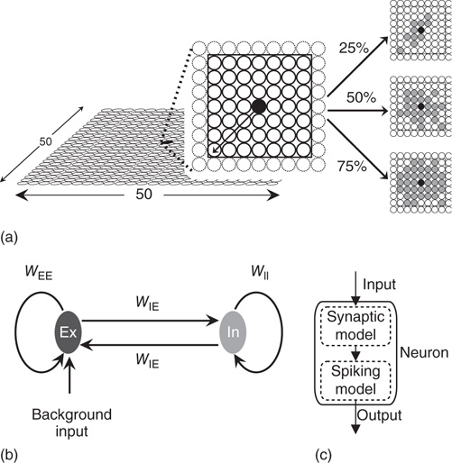
Figure 13.6 Structure of CROS model. (a) Neurons are situated in a 2D grid. A neuron (filled black circle) is connected in a local range (black box). Connectivity is defined as the percentage of connected neurons within this range. Shown in light gray to the right are the target neurons of example neurons with connectivity of 25% (top), 50% (middle), and 75% (bottom). (b) The network contains excitatory (Ex) and inhibitory (In) neurons, with connection weights (Wji) fixed depending on the type of the spiking (i) and receiving (j) neuron. (c) Each neuron consists of a synaptic model to integrate received spikes, and a spiking model.
13.6.1 CRitical OScillations Model (CROS)
The networks consisted of excitatory (75%) and inhibitory (25%) neurons arranged in an open grid, with local functional connectivity (Figure 13.6a). To define the local connectivity, each neuron was given a square area that marked the limits of being able to connect to other neurons. The connectivity probability for excitatory and inhibitory neurons was varied independently and is defined as the percentage of neurons that a neuron connects to within its local range. In neocortical tissue, local functional connectivity between neurons decays with distance; however, only a few empirical reports have assessed this quantitatively [62] [63]. Given the small radius of connectivity, this was implemented as an exponential decay.
Five networks were created for each combination of excitatory and inhibitory connectivity and each of these networks were simulated for 1000 s. The weights of these connections were dependent on the type (excitatory or inhibitory) of the presynaptic and postsynaptic neuron (Figure 13.6b), but were otherwise fixed in order to limit the number of free model parameters.
Neurons were modeled using a synaptic model integrating received spikes, and a probabilistic spiking model (Figure 13.6c). Each time step started with every neuron updating its synaptic model with received input. The spiking model is then updated by the synaptic model. On the basis of the spiking model, it is determined whether each neuron spikes. If a neuron spikes, the probability of spiking is reset, and this models a refractory period for the neuron. All neurons it connects to will receive an input from this neuron during the next time step.
13.6.2 CROS Produces Neuronal Avalanches with Balanced Ex/In Connectivity
The model displayed many forms of activity propagation depending on the excitatory/inhibitory connectivity ratio (Ex/In balance). This is illustrated in Figure 13.7A, where the temporal dynamics of activity propagation can be inferred from the color scale, indicating the time since a given neuron spiked. For the networks with a low Ex/In balance, the activity was characterized by localized wavelike spreading (Figure 13.7A-a). The propagation stops because of the strong local inhibition. With increasing Ex/In balance, the waves were able to spread further until they were able to reach across the entire network. In these networks, sustained activity patterns were possible (Figure 13.7A-b), with complex patterns such as spiral waves repeating themselves several times. These patterns would eventually dissipate with the network, either going through a period of low activity similar to the low Ex/In balance case or the network would become highly active and lose any spatially contiguous patterns. This highly active state is characteristic of the networks with a high Ex/In balance (Figure 13.7A-c).
The propagation of activity in the network was quantified using the concept of neuronal avalanches (Figure 13.7B), which have been reported for local field potential recordings in vitro [12] and in vivo [19]. The size of an avalanche is the total number of spikes during the avalanche, and the duration is the time spent with above-threshold activity. The size distributions were characterized using the statistical measure κ, which was developed by [64]. In agreement with visual inspection of the distributions, κ indicated that the model could produce subcritical, critical, or supercritical dynamics depending on the connectivity parameters (Figure 13.7C–F). The subcritical regime (κ < 1) had exponentially decaying avalanche sizes, the supercritical regime (κ > 1) had a characteristic scale indicated by the bump at large avalanche sizes, and power-law scaling extended up to the system size in the transition regime (κ ≈ 1).
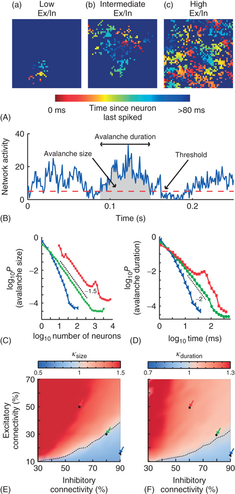
Figure 13.7 On short timescales (120 ms), activity spreads in the form of neuronal avalanches. (A) Example snapshot of network activity for three networks with different excitatory (Ex)/inhibitory (In) connectivity balance (Ex/In balance). Colors indicate the time since each neuron last spiked. (a) Networks with low Ex/In balance show wavelike propagation over short distances. (b) Networks with intermediate Ex/In balance often display patterns that are able to span the network and repeat. (c) Networks with high Ex/In balance have high network activity, but have little spatial coherence in their activity patterns. (B) An avalanche starts and ends when integrated network activity crosses a threshold value. (C) The avalanche-size distribution shows power-law scaling in the transition region (green circles) with a slope of −1.5 (dashed line). The subcritical region has an exponential distribution (blue triangles). The supercritical region (red squares) has a clear characteristic scale. (D) The avalanche-size distribution shows power-law scaling in the transition region (green circles) with a slope of −2 (dashed line). The subcritical region has an exponential distribution (blue triangles). The supercritical region (red squares) has a clear characteristic scale. (E) The connectivity-parameter space shows a transition (dashed black line) from subcritical (blue) to supercritical (red) avalanches. Arrows indicate the connectivity parameters of networks in (C). (F) The connectivity-parameter space shows a transition (dashed black line) from subcritical (blue) to supercritical (red) avalanches. Arrows indicate the connectivity parameters of networks in (D). (Modified from [61].)
13.6.3 CROS Produces Oscillations with LRTC When there are Neuronal Avalanches
On longer timescales (>120 ms), the progression of these avalanches gave the spatially integrated network activity a distinct oscillatory character (Figure 13.8A,B), which was qualitatively similar to what is typically observed in recordings of human resting-state MEG (Figure 13.8C) [59] [18]. Most network configurations produced 8–16 Hz oscillations (Figure 13.8D). To quantitatively assess scaling behavior on the level of oscillations, the waxing and waning of the oscillations (Figure 13.8B) were analyzed on the long timescales of 2–10 s using DFA (Figure 13.8E). In the model, DFA revealed a critical regime of strong temporal correlations (α = 1.0), whereas a relative increase in either inhibitory or excitatory connectivity led to reduced temporal correlations (α = 0.6), similar to those of filtered white noise (α = 0.5, Figure 13.8F). Interestingly, the binned averages of DFA exponents peaked when the network produced critical avalanches, with the correlations decreasing for the more subcritical or supercritical avalanches (Figure 13.8G). Taken together, the data indicated that nontrivial scaling behavior in the modulation of oscillatory activity can emerge on much longer timescales than those implemented in the model, and that neuronal avalanches may be viewed as the building blocks of neuronal oscillations with scale-free amplitude modulation.
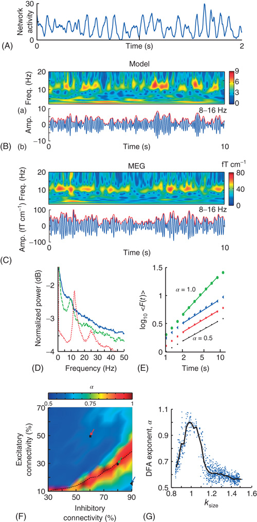
Figure 13.8 On long timescales (>2 s), the model produces oscillations qualitatively and quantitatively similar to human α-band oscillations. A: The spatially integrated network activity in a sliding window of 10 ms displays oscillatory variation. B: (a) Time-frequency plot of the integrated network activity from a network with 50% excitatory and 90% inhibitory connectivity. (b) Integrated network activity filtered at 8–16 Hz (blue), and the amplitude envelope (red). C: The same plots as in (B), but for a representative subject and MEG planar gradiometer above the parietal region. D: Power spectrum of the integrated network activity shows a clear peak frequency at ∼10 Hz for three networks with Excitatory:Inhibitory connectivity of 50% : 60% (red), 30% : 80% (green), and 15% : 90% (blue), respectively. E: DFA in double-logarithmic coordinates shows power-law scaling in the critical regime with α = 0.9 (green circles). The subcritical (α = 0.6, blue triangles) and supercritical (α = 0.6, red squares) regimes display similar correlations to a random signal (black dots). F: The connectivity-parameter space shows a clear peak region with stronger long-range temporal correlations. Overlaying the transition line from Figure 13.7E indicates that peak DFA occurs at κ ∼ 1. G: DFA exponents peak when the networks produce neuronal avalanches with critical exponents (κ ∼ 1). (Modified from [61].)
13.6.4 Multilevel Criticality: A New Class of Dynamical Systems?
The concept of multilevel criticality was proposed [61] to denote the phenomenon of critical behavior on multiple levels. Multilevel criticality may define a new class of dynamical systems, because it allows for criticality to emerge jointly on multiple levels separated by a characteristic scale, which is traditionally considered contradictory for critical dynamics.
The restricted spreading of activity in CRitical OScillations (CROS) seems essential for build up of temporal autocorrelations and criticality, as it allows clusters of nonexcitable and excitable neurons to form. These clusters act as memories of past activity, shaping the path of future activity analogously to a river's flow being shaped by the past flow of water [3] [65]. A recent study of model networks showed that a hierarchical topology can increase the range of parameters that give rise to critical dynamics – and thereby also the robustness of a critical state – because the modular topology limits activity spreading to local parts of the network [66]. Similarly, a localized topology is likely to support the emergence of oscillations with LRTCs.
Future research should address how multilevel criticality affects neuronal network properties such as its information processing capabilities, reactivity, ability to transiently synchronize with other networks, the importance of synaptic plasticity for these functional states to emerge and how memories are encoded, maintained, or lost in such networks.
Acknowledgment
The authors thank all the coworkers on the studies reviewed in the present chapter. In particular, Simon-Shlomo Poil, Teresa Montez, Giuseppina Schiavone, Rick Jansen, Vadim V. Nikulin, Dirk Smit, and Matias Palva.
References
- 1. Gilden, D.L. (2001) Cognitive emissions of 1/f noise. Psychol. Rev., 108 (1), 33–56.
- 2. Bassingthwaighte, J.B., Liebovitch, L.S. et al. (1994) Fractal Physiology, American Physiological Society by Oxford University Press, New York.
- 3. Bak, P. (1999) How Nature Works: The Science of Self-Organized Criticality, Copernicus Press, New York.
- 4. Goldberger, A.L., Amaral, L.A.N. et al. (2002) Fractal dynamics in physiology: alterations with disease and aging. Proc. Natl. Acad. Sci. U.S.A., 99, 1.
- 5. Stam, C. (2005) Nonlinear dynamical analysis of EEG and MEG: review of an emerging field. Clin. Neurophysiol., 116 (10), 2266–2301.
- 6. Ghosh, A., Rho, Y. et al. (2008) Noise during rest enables the exploration of the brain's dynamic repertoire. PLoS Comput. Biol., 4 (10), e1000196.
- 7. He, B.J., Zempel, J.M. et al. (2010) The temporal structures and functional significance of scale-free brain activity. Neuron, 66 (3), 353–369.
- 8. West, B.J. (2010) Frontiers: fractal physiology and the fractional calculus: a perspective. Front. Fractal Physiol., 1, 12.
- 9. Fries, P. (2005) A mechanism for cognitive dynamics: neuronal communication through neuronal coherence. Trends Cognit. Sci., 9 (10), 474.
- 10. Buzsáki, G. (2006) Rhythms of the Brain, Oxford University Press, New York.
- 11. Linkenkaer-Hansen, K., Nikouline, V.V. et al. (2001) Long-range temporal correlations and scaling behavior in human brain oscillations. J. Neurosci., 21 (4), 1370.
- 12. Beggs, J.M. and Plenz, D. (2003) Neuronal avalanches in neocortical circuits. J. Neurosci., 23 (35), 11167.
- 13. Haldeman, C. and Beggs, J.M. (2005) Critical branching captures activity in living neural networks and maximizes the number of metastable states. Phys. Rev. Lett., 94 (5), 58101.
- 14. Kinouchi, O. and Copelli, M. (2006) Optimal dynamical range of excitable networks at criticality. Nat. Phys., 2 (5), 348–351.
- 15. Levina, A., Herrmann, J.M. et al. (2007) Dynamical synapses causing self-organized criticality in neural networks. Nat. Phys., 3 (12), 857–860.
- 16. Plenz, D. and Thiagarajan, T.C. (2007) The organizing principles of neuronal avalanches: cell assemblies in the cortex? Trends Neurosci., 30 (3), 101–110.
- 17. Gireesh, E.D. and Plenz, D. (2008) Neuronal avalanches organize as nested theta-and beta/gamma-oscillations during development of cortical layer 2/3. Proc. Natl. Acad. Sci. U.S.A., 105 (21), 7576.
- 18. Poil, S., van Ooyen, A. et al. (2008) Avalanche dynamics of human brain oscillations: relation to critical branching processes and temporal correlations. Hum. Brain Mapping, 29 (7), 770.
- 19. Petermann, T., Thiagarajan, T.C. et al. (2009) Spontaneous cortical activity in awake monkeys composed of neuronal avalanches. Proc. Natl. Acad. Sci., 106 (37), 15921.
- 20. Chialvo, D.R. (2010) Emergent complex neural dynamics. Nat. Phys., 6 (10), 744–750.
- 21. Millman, D., Mihalas, S. et al. (2010) Self-organized criticality occurs in non-conservative neuronal networks during/up/'states. Nat. Phys., 6 (10), 801–805.
- 22. Rubinov, M., Sporns, O. et al. (2011) Neurobiologically realistic determinants of self-organized criticality in networks of spiking neurons. PLoS Comput. Biol., 7 (6), e1002038.
- 23. Bak, P., Tang, C. et al. (1987) Self-organized criticality: an explanation of the 1/f noise. Phys. Rev. Lett., 59 (4), 381.
- 24. Jensen, J. (1998). Self-Organized Criticality, H.J. Jensen, pp. 167, ISBN: 0521483719. Cambridge University Press: Cambridge, 1998.
- 25. Beggs, J. (2008) The criticality hypothesis: how local cortical networks might optimize information processing. Philos. Trans. Ser. A, Math. Phys. Eng. Sci., 366 (1864), 329.
- 26. Shew, W.L., Yang, H. et al. (2011) Information capacity and transmission are maximized in balanced cortical networks with neuronal avalanches. J. Neurosci.: Off. J. Soc. Neurosci., 31 (1), 55.
- 27. Gong, P., Nikolaev, A. et al. (2003) Scale-invariant fluctuations of the dynamical synchronization in human brain electrical activity. Neurosci. Lett., 336 (1), 33.
- 28. Kitzbichler, M.G., Smith, M.L. et al. (2009) Broadband criticality of human brain network synchronization. PLoS Comput. Biol., 5 (3), e1000314.
- 29. Monto, S., Vanhatalo, S. et al. (2007) Epileptogenic neocortical networks are revealed by abnormal temporal dynamics in seizure-free subdural EEG. Cereb. Cortex, 17 (6), 1386.
- 30. Atallah, B.V. and Scanziani, M. (2009) Instantaneous modulation of gamma oscillation frequency by balancing excitation with inhibition. Neuron, 62 (4), 566–577.
- 31. Rangarajan, G. and Ding, M. (2000) Integrated approach to the assessment of long range correlation in time series data. Phys. Rev. E, 61 (5), 4991.
- 32. Linkenkaer-Hansen, K., Smit, D.J.A. et al. (2007) Genetic contributions to long-range temporal correlations in ongoing oscillations. J. Neurosci., 27 (50), 13882–13889.
- 33. Hardstone, R., Poil, S.-S. et al. (2012) Detrended fluctuation analysis: a scale-free view on neuronal oscillations. Front. Physiol., 3.
- 34. Peng, C., Havlin, S. et al. (1995) Quantification of scaling exponents and crossover phenomena in nonstationary heartbeat time series. Chaos, 5 (1), 82–87.
- 35. Mandelbrot, B. (1967) How long is the coast of Britain? Statistical self-similarity and fractional dimension. Science, 156 (3775), 636.
- 36. Turcotte, D.L. (1997) Fractals and Chaos in Geology and Geophysics, Cambridge University Press, Cambridge.
- 37. Peitgen, H.O., Jurgens, H. et al. (1992) Chaos and Fractals: New Frontiers of Science, Springer, Berlin.
- 38. Eke, A., Hermán, P. et al. (2000) Physiological time series: distinguishing fractal noises from motions. Pflügers Arch.: Eur. J. Physiol., 439 (4), 403.
- 39. Eke, A., Herman, P. et al. (2002) Fractal characterization of complexity in temporal physiological signals. Physiol. Meas., 23, R1.
- 40. Beran, J. (1994) Statistics for Long-memory Processes, Chapman & Hall/CRC Press.
- 41. Mandelbrot, B.B. and Wallis, J.R. (1969) Some long-run properties of geophysical records. Water Resour. Res., 5 (2), 321–340.
- 42. Mandelbrot, B.B. (1982) The Fractal Geometry of Nature, Times Books.
- 43. Peng, C.K., Buldyrev, S.V. et al. (1994) Mosaic organization of DNA nucleotides. Phys. Rev. E, 49 (2), 1685.
- 44. Castiglioni, P., Parati, G. et al. (2010) Scale exponents of blood pressure and heart rate during autonomic blockade as assessed by detrended fluctuation analysis. J. Physiol., 589, 355–369.
- 45. Frey, U., Maksym, G. et al. (2011) Temporal complexity in clinical manifestations of lung disease. J. Appl. Physiol., 110 (6), 1723.
- 46. Hu, K., Ivanov, P.C. et al. (2001) Effect of trends on detrended fluctuation analysis. Phys. Rev. E, 64 (1), 011114.
- 47. Chen, Z., Ivanov, P.C. et al. (2002) Effect of nonstationarities on detrended fluctuation analysis. Phys. Rev. E Stat. Nonlinear Soft Matter Phys., 65 (4 Pt 1), 041107.
- 48. Xu, Y., Ma, Q.D.Y. et al. (2011) Effects of coarse-graining on the scaling behavior of long-range correlated and anti-correlated signals. Physica A: Stat. Mech. Appl., 390, 4057–4072.
- 49. Nikulin, V.V. and Brismar, T. (2005) Long-range temporal correlations in electroencephalographic oscillations: relation to topography, frequency band, age and gender. Neuroscience, 130 (2), 549–558.
- 50. Nikulin, V.V. and Brismar, T. (2004) Long-range temporal correlations in alpha and beta oscillations: effect of arousal level and test-retest reliability. Clin. Neurophys., 115 (8), 1896–1908.
- 51. Berthouze, L., James, L.M. et al. (2010) Human EEG shows long-range temporal correlations of oscillation amplitude in theta, alpha and beta bands across a wide age range. Clin. Neurophysiol., 121 (8), 1187–1197.
- 52. Smit, D.J.A., de Geus, E.J.C. et al. (2011) Scale-free modulation of resting-state neuronal oscillations reflects prolonged brain maturation in humans. J. Neurosci., 31 (37), 13128–13136.
- 53. Leopold, D.A., Murayama, Y. et al. (2003) Very slow activity fluctuations in monkey visual cortex: implications for functional brain imaging. Cereb. Cortex, 13 (4), 422.
- 54. Hohlefeld, F.U., Huebl, J. et al. (2012) Long-range temporal correlations in the subthalamic nucleus of patients with Parkinson's disease. Eur. J. Neurosci., 36, 2812–2821.
- 55. Linkenkaer-Hansen, K., Monto, S. et al. (2005) Breakdown of long-range temporal correlations in theta oscillations in patients with major depressive disorder. J. Neurosci., 25 (44), 10131–10137.
- 56. Montez, T., Poil, S.S. et al. (2009) Altered temporal correlations in parietal alpha and prefrontal theta oscillations in early-stage Alzheimer disease. Proc. Natl. Acad. Sci. U.S.A., 106 (5), 1614.
- 57. Nikulin, V.V., Jönsson, E.G. et al. (2012) Attenuation of long range temporal correlations in the amplitude dynamics of alpha and beta neuronal oscillations in patients with schizophrenia. Neuroimage, 61, 162–169.
- 58. Poil, S.S., Jansen, R. et al. (2011) Fast network oscillations in vitro exhibit a slow decay of temporal auto-correlations. Eur. J. Neurosci., 34, 394–403.
- 59. Linkenkaer-Hansen, K., Nikulin, V. et al. (2004) Stimulus-induced change in long-range temporal correlations and scaling behaviour of sensorimotor oscillations. Eur. J. Neurosci., 19 (1), 203.
- 60. Parish, L., Worrell, G. et al. (2004) Long-range temporal correlations in epileptogenic and non-epileptogenic human hippocampus. Neuroscience, 125 (4), 1069–1076.
- 61. Poil, S.-S., Hardstone, R. et al. (2012) Critical-state dynamics of avalanches and oscillations jointly emerge from balanced excitation/inhibition in neuronal networks. J. Neurosci., 32 (29), 9817–9823.
- 62. Holmgren, C., Harkany, T. et al. (2003) Pyramidal cell communication within local networks in layer 2/3 of rat neocortex. J. Physiol., 551 (Pt 1), 139.
- 63. Sporns, O. and Zwi, J. (2004) The small world of the cerebral cortex. Neuroinformatics, 2 (2), 145.
- 64. Shew, W., Yang, H. et al. (2009) Neuronal avalanches imply maximum dynamic range in cortical networks at criticality. J. Neurosci.: Off. J. Soc. Neurosci., 29 (49), 15595.
- 65. Chialvo, D.R. and Bak, P. (1999) Learning from mistakes. Neuroscience, 90 (4), 1137–1148.
- 66. Wang, S.J. and Zhou, C. (2012) Hierarchical modular structure enhances the robustness of self-organized criticality in neural networks. New J. Phys., 14 (2), 023005.