16
Criticality at Work: How Do Critical Networks Respond to Stimuli?

Mauro Copelli

Federal University of Pernambuco (UFPE), Physics Department, 50670-901, Recife-PE, Brazil

16.1 Introduction

Most models of critical neuronal networks have in common the theoretical ingredient of separation of time scales, according to which the interval between neuronal avalanches is much longer than their duration. This framework has proven useful for several reasons, among which are the possibilities of learning from an extensive literature on models of self-organized criticality and of comparing results with data obtained from some experimental setups. The brain of a freely behaving animal, however, is often found to operate away from this regime, thereby raising doubts about the relevance of criticality for brain function. In this chapter, two questions aimed at this direction are reviewed. From a theoretical perspective, how could criticality be harnessed by neuronal networks for processing incoming stimuli? From an experimental perspective, how could we know that the brain during natural behavior is critical?

In 2003, the idea that the brain (as a dynamical system) sits at (or fluctuates around) a critical point received compelling experimental support from Dietmar Plenz's lab: cortical slices show spontaneous activity in “bursts” with the very peculiar feature of not having a characteristic size. As described in the now-classic paper by Beggs and Plenz [1], the probability distributions of size () and duration () of these neuronal avalanches were experimentally measured and shown to be compatible with power laws, respectively, and . In the following, I will briefly review how this experimental result is connected with the theoretical idea of a critical brain (a much more expanded review can be found e.g., in Ref. [2]).

16.1.1 Phase Transition in a Simple Model

In order to do that, let us consider a very simple model of activity (e.g., spike) propagation in a network of connected neurons. We will make the drastic simplification that a neuron can be modeled by a finite set of states: if , neuron is in a quiescent state at time ; if , neuron is spiking; after a spike, the neuron deterministically goes through a number of refractory states, , and then returns to rest () (see Figure 16.1). In an excitable neuron, the transition from to does not occur spontaneously: model neurons spike only if somehow stimulated, either by an external stimulus (say, with probability ) or by synaptically connected neurons.

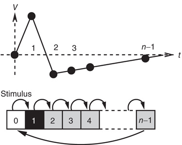
Figure 16.1 Toy model of an excitable neuron: “representative” values of the membrane potential are replaced by the discrete values of the cellular automaton (see text for details). Arrows denote transition probabilities, which are equal to except for the transition.

How do we model synaptic connections in such a simple model? Given a quiescent neuron , we look at all the neurons which are presynaptic to . Let us assume that noise in the system is such that the strength of the synaptic connection between a presynaptic neuron and postsynaptic neuron can be represented by the probability (another drastic simplification): if is quiescent () and is the only presynaptic neuron firing at time (), then, in the absence of external stimuli (), we have , where is the time step of the model (usually corresponding to ms, about the duration of a spike). If and several presynaptic neurons are firing, then . If we subject all neurons to this dynamics and update them synchronously, the model becomes a probabilistic cellular automaton whose evolution is governed by the connection matrix (see Figure 16.2). One of the advantages of such a simple model is that it allows one to simulate very large systems (say model neurons), even on a personal computer.

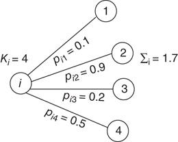
Figure 16.2 In this example, site has neighbors. One can define the local branching ratio , which gives the average number of “descendant” spikes that site would generate on its neighbors if they were all quiescent. The control parameter defined in the text is .

To render the model well defined, let us also postulate that neurons are randomly connected, that is, the network is an Erds–Rényi random graph. If we choose a symmetric connectivity matrix (definitely not a necessary ingredient), , and let (with drawn from a uniform distribution) and be, respectively, the average values of synaptic transmission probability and number of connections upon a neuron, then a convenient control parameter of the model is the so-called branching ratio . It can be thought of as approximately the average number of spikes that the neighbors of a spiking neuron will produce in the next time step if they are all currently quiescent. This model is essentially a variant of the one introduced by Haldeman and Beggs [3].

Let us keep the network without any external stimulus for the moment, . What happens if we initially allow a random fraction (say, 5% or 10%) of the neurons to be active, while the rest of them are quiescent? The activity of the initially active neurons will propagate (with some probability governed by ) to their quiescent neighbors, which will then propagate to their neighbors, and so forth. If , each spiking neuron will generate less than one spike in the subsequent time step, on average. So activity will tend to vanish with time: if all neurons become silent, the network will remain silent ever after (in the statistical physics literature, this is known as an absorbing state [4]). This is the so-called subcritical regime. For , however, each spike tends to be amplified, and activity will grow up to a certain limit, which is partly controlled by the refractory period of the neurons. This regime is called supercritical. The difference between and is therefore the stability of self-sustained activity in the network in the absence of any stimulus. It can be characterized by an order parameter, for instance, the density of active neurons averaged over time after an appropriate transient (i.e., the average firing rate).

What happens at ? For this value of the control parameter, the system undergoes a phase transition, where the order parameter departs continuously from zero () to nonzero values (). is the critical point at which the initial activity will also vanish but, differently from the subcritical regime, much more slowly, and without a characteristic time scale. The picture to have in mind is that of Figure 16.3.

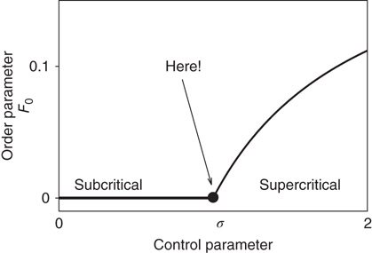
Figure 16.3 General picture of a second-order phase transition. An order parameter (here denoted by ) takes on nonzero values above a critical value of a control parameter (here denoted by ). In a second-order phase transition, the order parameter changes continuously at the critical point .

Details of the above model can be found in Ref. [5], where one can also find simple calculations that support the above conclusions. It is important to emphasize that some of the simplifications employed in this model cannot be taken for granted. The hand-waving argument for being the critical value of the coupling parameter, for instance, fails if the topology of the network is more structured than a simple Erds–Rényi random graph [6, 7]. The extension of the above results to more general topologies was put forward by Restrepo and collaborators [8, 9].

16.1.2 What is the Connection with Neuronal Avalanches?

Now that we have a simple model which very crudely mimics collective neuronal behavior, we can play with it and try to generate neuronal avalanches. Suppose we start in the subcritical regime, . We initially prepare the system by setting all neurons in the quiescent state. Then we randomly choose one neuron, make it fire, and see what happens. Activity will propagate to a certain extent but, since the system is subcritical, will eventually vanish. That means the avalanche we had started is over. We count the number of neurons that fired (in the model, that is the size of the avalanche) and keep it.

Now, only after the first avalanche is over do we create another one, repeating the procedure. It is important to emphasize that one of the pivotal theoretical ingredients of avalanche models is this clear separation of time scales, the interval between avalanches being much longer than their duration [10, 11]. We shall come back to this point later.

Going back to the subcritical regime, if we collect many avalanches and do the statistics, what we will find out is that avalanches have characteristic sizes and durations. That is, and decay exponentially for sufficiently large arguments. In other words, finding unusually large or long avalanches (i.e., much larger than the characteristic size or much longer than the characteristic time) is exponentially improbable.

The supercritical case, on the other hand, is very different. Although it is possible that a single firing neuron will generate an avalanche of finite size and duration, it is very likely that activity will propagate indefinitely (or for a very long time, which grows with the number of neurons in the model). Pragmatically, one has to set a limit on the maximum number of time steps one is willing to wait for an avalanche to end [12]. Once we repeat this procedure many times, we will obtain a distribution with a peak at a very large characteristic size.

At the critical point , simulations and calculations show that both the size and the duration distributions of the model avalanches obey power laws. For a number of topologies (including the simple Erds–Rényi random graph of our toy model), the exponents can be calculated [13, 14] and shown to be and , respectively.¹ These power laws and their exponents are in very good agreement with the experimental results obtained originally by Beggs and Plenz [1].

16.1.3 What if Separation of Time Scales is Absent?

The above-described power laws, which have been obtained at the critical point of a class of models, have been the main connection between the theory of critical phenomena and the experimental observation of neuronal avalanches. Let us recall that the connection relies heavily on the separation of time scales. In the experiments, the separation of time scales emerges naturally, not only in the original setup by Beggs and Plenz [1] but also in the cortex of anesthetized rats [19] and unanesthetized (but resting) monkeys [20]. In the models, the separation of time scales is typically imposed by hand,² that is, in the simulations one has to wait until an avalanche is over before creating another one.

But what if separation of time scales is absent? Consider, for instance, the cortical activity of a behaving animal, which typically does not display the separation of time scales seen under anesthesia or in reduced preparations. From a theoretical perspective, we could attempt to mimic such an ongoing activity by randomly stimulating our model network. In that case, how would the network respond, and what would be the role of criticality in the response? This question is addressed in Section 16.2.1.

From the perspective of an experimentalist, what would be the possible connections (if any) between the theory of critical phenomena and brain activity when there is no clear separation of time scales? A few tentative answers to this question will be reviewed in Section 16.2.2.

16.2 Responding to Stimuli

Physical stimuli impinge on our senses and get translated into neuronal activity, which is then further processed in many steps, eventually allowing us to make (some) sense of the world. In the context of the study of sensory systems, therefore, the question of how neurons respond to stimuli is natural and has a very long history (see e.g., [24, 25]). Here we would like to explore our simple model to make the case that, in some well-defined sense, the network collectively responds optimally if it is at criticality.

16.2.1 What Theory Predicts

Let us revisit our toy model, now relaxing the condition . If , neurons can also fire “spontaneously.” We have employed this simple framework to model the interaction between physical stimuli and sensory neurons, by assuming that is an increasing function of the intensity of the stimulus [26–29]. In what follows, we employ , where is a Poisson rate assumed to be proportional to the stimulus intensity. Neurons are assumed to be stimulated independently.

How does that scenario compare with that in which avalanches were obtained? Once , separation of time scales is lost, since the network is constantly being stimulated. At every time step, a quiescent neuron may fire with nonzero probability because of an external stimulus, whether or not a spike was propagated from a spiking neighbor. One can think of this scenario as though several avalanches were being generated at every time step. Each of them then spreads out, a process that, as we have seen, is controlled by the coupling parameter . And they may interact nonlinearly with one another. If we look beyond the current model, in a more general scenario we are randomly generating spatio-temporal bursts of activity in an excitable medium. Loosely speaking, avalanches in this model are excitable waves in a probabilistic, excitable medium which has been tuned to its critical point.

16.2.1.1 Self-Regulated Amplification via Excitable Waves

In the context of sensory processing, how could the activity of our model network convey information about the physical stimulus impinging on it? Historically, the simplest assumption has been the so-called rate coding, namely, that the mean neuronal activity could somehow represent the stimulus rate [25]. Let be the mean firing rate of the network and be its response function. How do we expect to change as we go from subcritical () to critical () and then to a supercritical () regime?

Let us begin with the subcritical case, a quiescent network, and small . For very small (say, ), whenever a model neuron is externally stimulated, it generates an excitable wave which is likely to be small and to evanesce after propagating across a few synapses. So, for each instance the Poisson process happens to stimulate the network (at rate ), the average response is a small number of spikes. In the context of the rate coding mentioned above, that means that the coupling among the neurons manages to somehow amplify the signal that impinged upon a single neuron. Without the coupling (), the same stimulus would have generated a single spike in our model excitable neuron. One can in fact define an amplification factor [26].

If we increase slightly, the process described above simply occurs more often across the network, but for sufficiently small and the excitable waves essentially do not interact. This reasoning suggests that increases linearly for small and small , which is exactly what a simple mean-field calculation confirms [5]. Note that the larger the , the larger the probability of propagation and the larger the size of the resulting evanescent excitable wave. Therefore, increasing leads to a stronger amplification of the incoming signals. These linear response curves for low stimulus are shown in the lower curves of Figure 16.4a,b (log–log plot and lin–log plot, respectively).

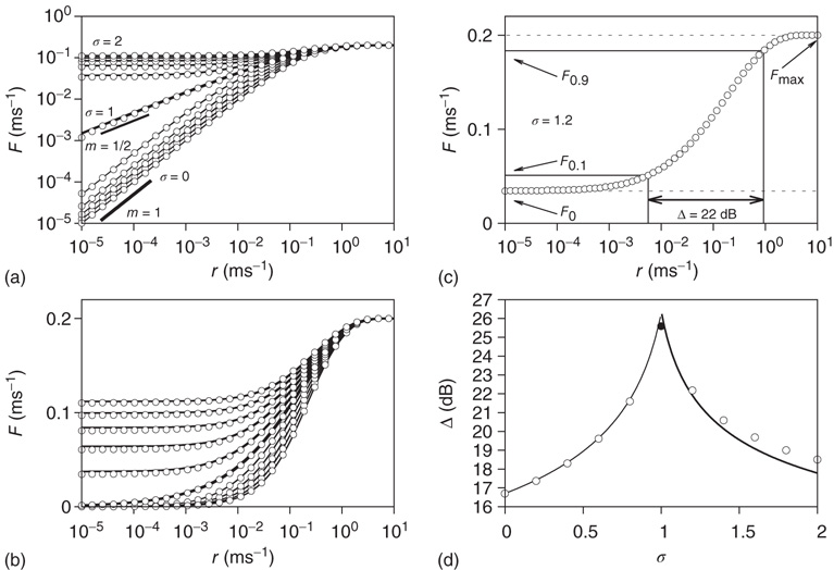
Figure 16.4 (a) Response functions with increasing from bottom to top, in log–log scale. The exponent shows that the low-stimulus response is linear in the subcritical case () and nonlinear in the critical case (). (b) Same as (a), except for the lin–log scale. (c) How to calculate the dynamic range of a response curve (see text for details). (d) Dynamic range as a function of coupling.

(Adapted from Ref. [5].)

On increasing sufficiently, excitable waves will be created often and close enough so as to interact. When this happens, the nonlinearities of an excitable medium play a very interesting role. For the sake of reasoning, consider initially a one-dimensional chain of excitable neurons and two deterministic counterpropagating excitable waves on it. The site at which the waves meet is initially quiescent, but will be excited by both its left and right spiking neighbors. After that, the excitation of the collision point cannot go anywhere, because both the left and right neighbors are refractory [26]. Therefore, upon collision, excitable waves annihilate each other (differently from waves in a linear medium, such as light in vacuum). In more than one dimension, the phenomenon is not so simple, because the wave fronts can have many different shapes (sometimes fractal) and typically intersect partially with one another. Nonetheless, the annihilation persists at whichever site they happen to bump into one another. An important consequence is, therefore, that, for large , amplification of incoming signals by propagation of excitable waves is severely limited by the annihilation of the excitable waves. Thus for strong stimuli, the coupling among neurons does not change much the average firing rate . This can be seen again in Figure 16.4a,b, where the curves converge to the same saturation response (including the uncoupled case ) for large .

Therefore, we arrive at this very appealing result: for weak stimuli (small ), amplification is large (the larger the coupling , the larger the amplification); for strong stimuli (large ), amplification is small (i.e., the amplification factor is a decreasing function of [26]). In other words, amplification of the incoming signals is self-regulated, a phenomenon that emerges naturally from very basic properties of excitable media.

16.2.1.2 Enhancement of Dynamic Range

Intuitively, amplifying weak stimuli while not amplifying strong stimuli looks like a good strategy for further processing of the incoming signals. The dynamic range is a standard and simple concept that somehow quantifies how good this strategy is.

Consider the response function exemplified in Figure 16.4c, which has a baseline activity for and saturates at for . Near those two plateau levels, the response does not change much as we vary . If we knew the firing rate and had to use this knowledge to infer the intensity of the incoming stimulus (i.e., invert the function ), the task would be very difficult if was close to or .

Let us define and according to , as shown in the horizontal lines of Figure 16.4(c). These firing rate values are sufficiently distant from the plateaus such that, for , it is reasonable to state that we can obtain if we know (the 10% and 90% levels are arbitrary but standard in the literature, see e.g., Ref. [30]). In other words, if we define such that , then the stimulus rates in the interval (marked by vertical lines in Figure 16.4c) are reasonably “coded by” . The dynamic range is the range of stimuli, measured in decibels, within this interval:

16.1

In the example of Figure 16.4c, the dynamic range covers 2.2 decades of stimulus intensity.

Note that, operationally, can be understood as the network sensitivity level above which stimulus intensities are “detected.” The network sensitivity depends strongly on , thanks to the amplification via excitable waves. The upper value , on the other hand, is only weakly affected. We therefore conclude that the benefits of self-limited amplification discussed above are well captured by the dynamic range: as shown in the left region of Figure 16.4d, increases with in the subcritical regime.

This result is very robust because, as mentioned previously, it depends on very few properties of excitable media. Enhancement of dynamic range has been observed in models which in their details are very different from the one described in Section 16.1.1, from deterministic excitable media (one- [26, 29], two- [27, 28, 31] and three-dimensional networks [31]) to a detailed conductance-based model of the retina [32]. In fact, one can look at a smaller scale and consider the dendritic tree of a single neuron. If the dendrites are active, dendritic spikes can propagate along the branches, a phenomenon whose significance has challenged the field of so-called dendritic computation [33]. By regarding an active dendritic tree as an excitable medium with a tree-like topology, enhancement of neuronal dynamic range emerges as a robust property, both in a simple cellular automaton [34, 35] and in a more sophisticated conductance-based model on top of morphologically reconstructed dendrites [36].

16.2.1.3 Nonlinear Collective Response and Maximal Dynamic Range at Criticality

What happens if we increase to its critical value? At the critical point, the theory of critical phenomena predicts that the low-stimulus response function is governed by another critical exponent [4], namely

16.2

Our model is amenable to mean-field calculations, yielding [5], a nonlinear, power-law response which is shown in Figure 16.4a,b. The exponent can be different for more structured topologies [15, 37] and deterministic models [31, 38], but the fact that it is always less than unity means that low-stimulus response is amplified and dynamic range is enhanced at the critical point (as compared to a linear response in the subcritical regime).

If we increase further and reach the supercritical regime, the benefits of low-stimulus amplification begin to deteriorate. In that regime, the same coupling that amplifies weak stimuli via propagation of excitable waves also renders those waves long-lasting, so that self-sustained activity becomes stable. The network now has a baseline activity with which the response to a weak stimulus is mixed and from which it is hard to discern. This situation is shown in the upper lines of Figure 16.4a,b. The situation is analogous to someone whispering on a microphone connected to an overamplified system dominated by audio feedback. The larger the coupling , the larger the network self-sustained activity (see Figure 16.3), which implies that the dynamic range is a decreasing function of in the supercritical regime.

Figure 16.4d summarizes the above discussion: the dynamic range attains its maximum at criticality. Of all the possible values of the coupling strength, the sensory network responds optimally at . Moreover, we can go back to our original question of Section 16.1.3: without separation of time scales in the network activity, how could one tell whether the system is at criticality? One potential fingerprint is shown in Figure 16.4b: at criticality, the low-stimulus response function is a power law, with an exponent less than unity (see Eq. (16.2)).

In hindsight, the reasoning underlying Figure 16.4d is straightforward. The ability to process stimulus intensities across several orders of magnitude is maximal at the point where stimuli are amplified as much as possible, but not so much as to engage the network in stable self-sustained activity. That result has been generalized in a number of models, including excitable networks with scale-free topology [6, 7], with signal integration where discontinuous transitions are possible [39], or with an interplay between excitatory and inhibitory model neurons [40]. In fact, the mechanism does not even need to involve excitable waves, appearing also in a model of olfactory processing where a disinhibition transition involving inhibitory units takes place [41].

16.2.2 What Data Reveals

Our simple model predicts that a system at criticality responds to stimuli (i) nonlinearly and (ii) with maximal dynamic range. Let us now briefly review how these predictions compare with experimental data.

16.2.2.1 Nonlinear Response Functions in Sensory Systems

The oldest reports of a nonlinear power law response to sensory stimuli probably come from psychophysics, a field founded in the nineteenth century. Steven's psychophysical law states that the psychological sensation of a physical stimulus with intensity is a power law , where is the Stevens exponent [42]. Since the intensity of physical stimuli varies by several orders of magnitude, it is not surprising that psychophysical responses have a large dynamic range, with Stevens exponents usually taking values less than : for light intensity of a point source, whereas for the smell of heptane [42], for instance.

On the one hand, it is remarkable that the values of Stevens exponents are so close to the ones obtained from simple models, given that psychophysical responses involve a plethora of brain regions for the processing of sensory information. On the other hand, it has been argued that the nonlinear transduction of physical stimuli must be done at the sensory periphery to prevent early saturation [42], in which case the simple models would need to mimic only the first processing layers [5, 26–29, 31].

In fact, power law responses to stimuli are indeed observed at a smaller scale in early sensory processing. Odorant-evoked fluorescence activity in olfactory glomeruli of the mouse follows a power law relation with odorant concentration [43]. In the mouse retina, the spiking response of ganglion cells to visual stimulus [44] can be reasonably well fitted by a power law with exponent [29]. The highly nonlinear response observed in projection neurons of the antennal lobe of the fruit fly also seems consistent with a power law [45].

16.2.2.2 Enhanced Dynamic Range

In our simple model, the strength of the coupling between neurons and is simply a probability , a drastic simplification in which we project our ignorance of the many mechanisms governing the propensity for the th neuron to fire, given that the th did. In an experiment, several mechanisms could mediate the putative amplification via excitable waves that we have described, and the enhancement of dynamic range that ensues.

One of these mechanisms could be the electrical coupling among neurons via electrical synapses (gap junctions). In the experimental setup of Deans et al. [44], the response of retinal ganglion cells has its dynamic range reduced from 23 dB in wild-type mice to 14 dB in connexin36 knockouts [29]. The role of lateral electrical coupling in enhancing sensitivity is also consistent with the upregulation of connexin36 in dark-adapted chicks [46] as well as with detailed simulations of the vertebrate retina [32, 36].

In the cortex, the balance between excitation and inhibition is mediated mostly by chemical synapses. Shew et al. [12] have recorded the activity of cortex slice cultures via microelectrode arrays. They could pharmacologically change the ratio of excitation and inhibition via the application of antagonists of glutamatergic or GABAergic synaptic transmission. After the application of an electrical pulse of variable intensity (the stimulus) in one of the electrodes, they measured the collective response of the slice. What they found is that, averaging over several slices, the dynamic range of the response function was maximal for the no-drug condition. When the system was made more insensitive (by reducing excitatory synaptic transmission) or more hyperexcitable (by reducing inhibitory synaptic transmission), in either case the dynamic range was reduced. Moreover, for each slice the dynamic range was maximal whenever the avalanche size distribution was compatible with a power law [12].

16.2.2.3 Scaling In Brain Dynamics

Although the dynamic range is a natural quantity to be considered in the context of sensory systems, there are many situations in which it can be very difficult to measure, or simply not relevant. Alternative fingerprints of criticality have been proposed for these cases. For instance, nontrivial scaling properties are predicted to appear in the distributions describing critical phenomena [47]. In this scenario, power law distributions of the size and duration of neuronal avalanches are but one example of scale invariance.

At the behavioral level, several interesting results have been obtained. For instance, sleep–wake transitions have been shown to be governed by power law distributions across mammalian species, suggesting scale-invariant features in the mechanisms of sleep control [48]. Nontrivial scaling properties have also been found in the fluctuations of the motor activity of rats, with power laws governing the distribution of time intervals between consecutive movements [49].

Ribeiro et al. relied on similar tools to analyze in vivo brain activity at the scale of a multielectrode array, with which spike avalanches were recorded from the cerebral cortex and hippocampus of rats [50]. Power law size distributions appeared only under anesthesia (a result reminiscent of those observed in dissociated neurons[51, 52]). When rats were freely behaving, no clear separation of time scales was seen in spiking activity, as shown in Figure 16.5a [50].

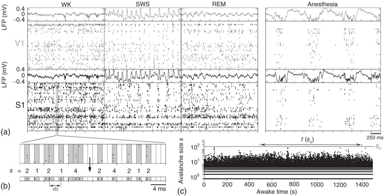
Figure 16.5 (a) Raster plot and local field potential (LFP) traces from two brain regions (V1 and S1) of a freely behaving rat during the three major behavioral states. (left panels: waking = WK, slow-wave sleep = SWS and rapid-eye-movement sleep = REM) and during anesthesia (right panel). (b) Operational definition of avalanche: the mean inter-event interval (IEI) is calculated taking into account all neurons and then is used as the time bin. This example shows avalanches of sizes (c) Time series of avalanche sizes for a WK window. denotes one instance of the waiting time between avalanches of size , from which the distribution of inter-avalanche intervals is then calculated (see text for details).

(Adapted from Ref. [50].)

Employing an operational definition of avalanches with rate-normalized time bins (see Figure 16.5b), Ribeiro et al. obtained avalanche sizes spanning at least two orders of magnitude, as shown in Figure 16.5c. The size distributions were well fitted by lognormals instead of power laws, as shown in Figure 16.6 (upward triangles). In an attempt to verify whether this result necessarily invalidated the hypothesis of a critical brain, a two-dimensional cellular automaton (otherwise similar to the one described in Section 16.1.1) was simulated at the critical point, yielding a power law size distribution (Figure 16.6, circles). Then, avalanches were deliberately undersampled with a spatial structure equivalent to the multielectrode array that gave rise to the data (see inset of Figure 16.6). Even though the model was critical, the simulated avalanches exhibited size distributions compatible with lognormals when undersampled (Figure 16.6, downward triangles), in close agreement with the experimental data [50]. As had been previously shown by Priesemann et al., avalanche size distributions can change considerably if a critical system is partially sampled [53]. Therefore, the lack of a power law distribution in an undersampled system does not mean that the system is not critical.

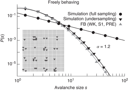
Figure 16.6 Distribution of avalanche sizes for a freely behaving rat (upward triangles) fit by a lognormal function; simulations of a two-dimensional model at criticality (circles) and a power law fit with exponent ; simulations of the same model, but from avalanches measured only at a subset of the sites (downward triangles), as depicted in the inset (the underlying line is also a lognormal fit).

(Adapted from Ref. [50].)

Ribeiro et al. also explored fingerprints of criticality in the time domain. Consider the time series of avalanche sizes shown in Figure 16.5V. First, long-range time correlations were observed in spectra and detrended fluctuation analysis (DFA) exponents close to [50]. Second, the probability density function of waiting times between consecutive avalanches of size was well described by a scaling function. The left column of Figure 16.7a shows a family of such distributions, where each color denotes a different value of size . The larger the required size , the longer one typically has to wait before an avalanche occurs, leading to heavier and heavier tails as increases. Let be the average waiting time for a given value of . If we then plot a normalized density versus a normalized time , the family of curves for all values of collapses onto a single function. As shown in Figure 16.7a, the collapse spans about six orders of magnitude. Moreover, since the rescaled axes are dimensionless, different animals could be compared. As it turns out, a single scaling function fits the data across animals, across brain regions, and across behavioral states [50]. This scaling function is a double power law, with exponents similar to those observed in other systems believed to be critically self-organized [54]. Taken together, the results suggest a universal mechanism underlying the dynamics of spike avalanches in the brain. In anesthetized animals, however, the same kind of scaling does not seem to hold (see Figure 16.7b), despite the fact that power law size distributions appear in that case [50].

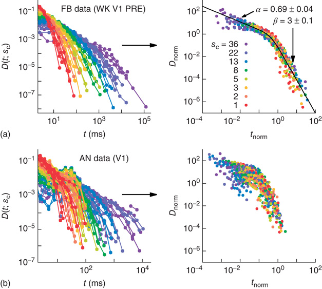
Figure 16.7 Families of distributions of inter-avalanche intervals for (a) freely behaving animals and (b) anesthetized animals. Left column: regular distributions. Right column: rescaled distributions (see text for details). Different colors denote different values of . (Adapted from Ref. [50].)

16.3 Concluding Remarks

We have reviewed the basic connection between criticality in a class of simple models and the experimentally observed power law size distributions of neuronal avalanches. Separation of time scales is an important ingredient for that connection, appearing naturally in reduced preparations and being usually imposed by construction in models.

Absent that ingredient, other features emerge as potential signatures of criticality. The response function of a model network to weak stimuli has prominent features at criticality: it is nonlinear, a power law with an exponent less than . It also has maximal dynamic range. We have reviewed some experimental results that seem consistent with those features. It is important to emphasize that, besides the dynamic range, other interesting quantities such as information storage and transmission are maximized at criticality, as recently reviewed by Shew and Plenz [55].

The scaling properties expected at criticality have also provided a number of tools with which to analyze data. Temporal aspects, in particular, pose challenges for modeling which are now being addressed. Poil et al. have recently proposed a model which displays power law size distribution of avalanches as well as long-range time correlations (as measured by DFA exponents) [22]. The nonmonotonic distribution of avalanche waiting times seen in slices has also been recently modeled by Lombardi et al. [23].

The simple model described in Section 16.1.1 amounts essentially to a branching process on top of a random graph. The transition in these models between an active and an absorbing phase has been very helpful in that it yields exponents for the power laws in the distributions of size and duration which are compatible with those observed experimentally. However, these are mean-field exponents, which in principle can be obtained by several other models. In other words, in the simplest scenario where separation of time scales is imposed by hand, these simple models are somewhat limited in what they can predict. Currently, we cannot be sure that the phase transition exhibited by these models (absorbing active) is to a reasonable first approximation of the one taking place in the brain. So the search for new measures (scaling properties, adequate order parameters, etc.) with which to characterize criticality in the brain remains a fascinating challenge to be embraced by experimentalists and theoreticians alike.

Acknowledgements

This chapter is but a brief summary of work that has been performed over the years with many collaborators, with whom I am glad to share the credit and to whom I am deeply thankful. An incomplete list includes Osame Kinouchi, Sidarta Ribeiro, Paulo R. A. Campos, Antonio C. Roque and Dante R. Chialvo, as well as (and most specially) my students and former students Lucas S. Furtado, Tiago L. Ribeiro, Vladimir R. V. Assis, and Leonardo L. Gollo. I also thank Dietmar Plenz and Ernst Niebur for their efforts in organizing the wonderful conference which gave rise to this book. Financial support for the research by me reported in this chapter is gratefully acknowledged and was provided by Brazilian agencies CNPq, FACEPE and CAPES, as well as special programs PRONEX, PRONEM and INCeMaq.

References

1. 1. Beggs, J.M. and Plenz, D. (2003) Neuronal avalanches in neocortical circuits. J. Neurosci., 23 (35), 11 167.
2. 2. Chialvo, D. (2010) Emergent complex neural dynamics. Nat. Phys., 6 (10), 744–750.
3. 3. Haldeman, C. and Beggs, J.M. (2005) Critical branching captures activity in living neural networks and maximizes the number of metastable states. Phys. Rev. Lett., 94 (5), 58 101.
4. 4. Marro, J. and Dickman, R. (1999) Nonequilibrium Phase Transition in Lattice Models, Cambridge University Press.
5. 5. Kinouchi, O. and Copelli, M. (2006) Optimal dynamical range of excitable networks at criticality. Nat. Phys., 2, 348–352.
6. 6. Copelli, M. and Campos, P.R.A. (2007) Excitable scale-free networks. Eur. Phys. J. B, 56, 273–278.
7. 7. Wu, A., Xu, X., and Wang, Y. (2007) Excitable Greenberg-Hastings cellular automaton model on scale-free networks. Phys. Rev. E, 75 (3), 032 901.
8. 8. Larremore, D.B., Shew, W.L., and Restrepo, J.G. (2011a) Predicting criticality and dynamic range in complex networks: effects of topology. Phys. Rev. Lett., 106, 058101.
9. 9. Larremore, D.B., Shew, W.L., Ott, E., and Restrepo, J.G. (2011) Effects of network topology, transmission delays, and refractoriness on the response of coupled excitable systems to a stochastic stimulus. Chaos, 21 (2), 025117.
10. 10. Bak, P., Tang, C., and Wiesenfeld, K. (1987) Self-organized criticality: an explanation of 1/f noise. Phys. Rev. Lett., 59 (4), 381–384.
11. 11. Bak, P. (1996) How Nature Works: The Science of Self-Organized Criticality, Springer, New York.
12. 12. Shew, W., Yang, H., Petermann, T., Roy, R., and Plenz, D. (2009) Neuronal avalanches imply maximum dynamic range in cortical networks at criticality. J. Neurosci., 29, 15 595.
13. 13. Harris, T. (1963) The Theory of Branching Processes, Springer.
14. 14. Larremore, D.B., Carpenter, M.Y., Ott, E., and Restrepo, J.G. (2012) Statistical properties of avalanches in networks. Phys. Rev. E Stat. Nonlin. Soft Matter Phys., 85 (6).
15. 15. Muñoz, M.A., Dickman, R., Vespignani, A., and Zapperi, S. (1999) Avalanche and spreading exponents in systems with absorbing states. Phys. Rev. E, 59 (5), 6175.
16. 16. Hinrichsen, H. (2009) Observation of directed percolation - a class of nonequilibrium phase transitions. Physics, 2, 96.
17. 17. Takeuchi, K.A., Kuroda, M., Chaté, H., and Sano, M. (2007) Directed percolation criticality in turbulent liquid crystals. Phys. Rev. Lett., 99 (23), 234–503.
18. 18. Takeuchi, K.A., Kuroda, M., Chaté, H., and Sano, M. (2009) Experimental realization of directed percolation criticality in turbulent liquid crystals. Phys. Rev. E, 80 (5), 051–116.
19. 19. Gireesh, E.D. and Plenz, D. (2008) Neuronal avalanches organize as nested theta-and beta/gamma-oscillations during development of cortical layer 2/3. Proc. Natl. Acad. Sci. U.S.A., 105 (21), 7576.
20. 20. Petermann, T., Thiagarajan, T.C., Lebedev, M.A., Nicolelis, M.A.L., Chialvo, D.R., and Plenz, D. (2009) Spontaneous cortical activity in awake monkeys composed of neuronal avalanches. Proc. Natl. Acad. Sci. U.S.A., 106 (37), 15 921.
21. 21. Millman, D., Mihalas, S., Kirkwood, A., and Niebur, E. (2010) Self-organized criticality occurs in non-conservative neuronal networks during Up states. Nat. Phys., 6 (10), 801–805.
22. 22. Poil, S.S., Hardstone, R., Mansvelder, H.D., and Linkenkaer-Hansen, K. (2012) Critical-state dynamics of avalanches and oscillations jointly emerge from balanced excitation/inhibition in neuronal networks. J. Neurosci., 32 (29), 9817–9823.
23. 23. Lombardi, F., Herrmann, H., Perrone-Capano, C., Plenz, D., and de Arcangelis, L. (2012) Balance between excitation and inhibition controls the temporal organization of neuronal avalanches. Phys. Rev. Lett., 108 (22), 228 703.
24. 24. Adrian, E.D. (1926) The impulses produced by sensory nerve endings. Part 1. J. Physiol., 61, 49–72.
25. 25. Rieke, F., Warland, D., de Ruyter van Stevenink, R.R., and Bialek, W. (1996) Spikes: Exploring the Neural Code, MIT Press.
26. 26. Copelli, M., Roque, A.C., Oliveira, R.F., and Kinouchi, O. (2002) Physics of Psychophysics: Stevens and Weber-Fechner laws are transfer functions of excitable media. Phys. Rev. E, 65 (6), 060 901.
27. 27. Copelli, M., Oliveira, R.F., Carlos Roque, A., and Kinouchi, O. (2005) Signal compression in the sensory periphery. Neurocomputing, 65, 691–696.
28. 28. Copelli, M. and Kinouchi, O. (2005) Intensity coding in two-dimensional excitable neural networks. Physica A, 349 (3), 431–442.
29. 29. Furtado, L.S. and Copelli, M. (2006) Response of electrically coupled spiking neurons: a cellular automaton approach. Phys. Rev. E, 73 (1), 011 907.
30. 30. Rospars, J.P., Lánsky, P., Duchamp-Viret, P., and Duchamp, A. (2000) Spiking frequency versus odorant concentration in olfactory receptor neurons. BioSystems, 58 (1), 133–141.
31. 31. Ribeiro, T.L. and Copelli, M. (2008) Deterministic excitable media under poisson drive: power law responses, spiral waves, and dynamic range. Phys. Rev. E, 77 (5), 051 911.
32. 32. Publio, R., Oliveira, R.F., and Roque, A.C. (2009) A computational study on the role of gap junctions and rod ih conductance in the enhancement of the dynamic range of the retina. PloS One, 4 (9), e6970.
33. 33. Stuart, G., Spruston, N., and Häusser, M. (1999) Dendrites, Oxford University Press.
34. 34. Gollo, L.L., Kinouchi, O., and Copelli, M. (2009) Active dendrites enhance neuronal dynamic range. PLoS Comput. Biol., 5 (6), e1000 402.
35. 35. Gollo, L.L., Kinouchi, O., and Copelli, M. (2012a) Statistical physics approach to dendritic computation: the excitable-wave mean-field approximation. Phys. Rev. E, 85 (1), 011 911.
36. 36. Publio, R., Ceballos, C.C., and Roque, A.C. (2012) Dynamic range of vertebrate retina ganglion cells: importance of active dendrites and coupling by electrical synapses. PloS One, 7 (10), e48 517.
37. 37. Assis, V.R. and Copelli, M. (2008) Dynamic range of hypercubic stochastic excitable media. Phys. Rev. E, 77 (1), 011 923.
38. 38. Ohta, T. and Yoshimura, T. (2005) Statistical pulse dynamics in a reaction–diffusion system. Physica D, 205 (1), 189–194.
39. 39. Gollo, L.L., Mirasso, C., and Eguíluz, V.M. (2012b) Signal integration enhances the dynamic range in neuronal systems. Phys. Rev. E, 85 (4), 040 902.
40. 40. Pei, S., Tang, S., Yan, S., Jiang, S., Zhang, X., and Zheng, Z. (2012) How to enhance the dynamic range of excitatory-inhibitory excitable networks. Phys. Rev. E, 86 (2), 021 909.
41. 41. Buckley, C.L. and Nowotny, T. (2011) Multiscale model of an inhibitory network shows optimal properties near bifurcation. Phys. Rev. Lett., 106 (23), 238 109.
42. 42. Stevens, S. (1975) Psychophysics: Introduction to its Perceptual, Neural and Social Prospects, John Wiley & Sons, Inc., New York.
43. 43. Wachowiak, M. and Cohen, L.B. (2001) Representation of odorants by receptor neuron input to the mouse olfactory bulb. Neuron, 32 (4), 723–735.
44. 44. Deans, M.R., Volgyi, B., Goodenough, D.A., Bloomfield, S.A., and Paul, D.L. (2002) Connexin36 is essential for transmission of rod-mediated visual signals in the mammalian retina. Neuron, 36 (4), 703–712.
45. 45. Bhandawat, V., Olsen, S.R., Gouwens, N.W., Schlief, M.L., and Wilson, R.I. (2007) Sensory processing in the drosophila antennal lobe increases reliability and separability of ensemble odor representations. Nat. Neurosci., 10 (11), 1474–1482.
46. 46. Kihara, A., Paschon, V., Cardoso, C., Higa, G., Castro, L., Hamassaki, D., and Britto, L. (2009) Connexin36, an essential element in the rod pathway, is highly expressed in the essentially rodless retina of gallus gallus. J. Comp. Neurol., 512 (5), 651–663.
47. 47. Sornette, D. (2000) Critical Phenomena in Natural Sciences, Springer.
48. 48. Lo, C.C., Chou, T., Penzel, T., Scammell, T.E., Strecker, R.E., Stanley, H.E., and Ivanov, P.C. (2004) Common scale-invariant patterns of sleep–wake transitions across mammalian species. Proc. Natl. Acad. Sci. U.S.A., 101 (50), 17545.
49. 49. Anteneodo, C. and Chialvo, D. (2009) Unraveling the fluctuations of animal motor activity. Chaos, 19 (3), 033123.
50. 50. Ribeiro, T., Copelli, M., Caixeta, F., Belchior, H., Chialvo, D., Nicolelis, M., and Ribeiro, S. (2010) Spike avalanches exhibit universal dynamics across the sleep-wake cycle. PloS One, 5 (11), e14 129.
51. 51. Mazzoni, A., Broccard, F.D., Garcia-Perez, E., Bonifazi, P., Ruaro, M.E., and Torre, V. (2007b) On the dynamics of the spontaneous activity in neuronal networks. PloS One, 2 (5), e439.
52. 52. Pasquale, V., Massobrio, P., Bologna, L., Chiappalone, M., and Martinoia, S. (2008) Self-organization and neuronal avalanches in networks of dissociated cortical neurons. Neuroscience, 153 (4), 1354–1369.
53. 53. Priesemann, V., Munk, M.H., and Wibral, M. (2009) Subsampling effects in neuronal avalanche distributions recorded in vivo. BMC Neurosci., 10 (1), 40.
54. 54. Bak, P., Christensen, K., Danon, L., and Scanlon, T. (2002) Unified scaling law for earthquakes. Phys. Rev. Lett., 88 (17), 178 501.
55. 55. Shew, W.L. and Plenz, D. (2013) The functional benefits of criticality in the cortex. Neuroscientist, 19 (1), 88–100.

¹ These are the mean-field critical exponents for the models belonging to the directed percolation (DP) universality class. For models on this universality class running on more structured, hypercubic lattices, the exponents are different [15]. As a historical note, it is interesting that it has taken over 50 years for these DP exponents to be experimentally observed in physical systems [16–18].

² save for a few notable exceptions, see, for example, Refs. [21–23].