17
Critical Dynamics in Complex Networks
17.1 Introduction: Critical Branching Processes
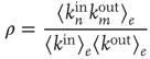
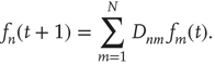
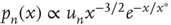
A central concept in the preceding chapters has been that of a critical branching process that has been used to explain the statistics of neuronal avalanches observed in vivo and in vitro. Branching processes were first systematically studied by Galton and Watson [1] in 1874 in a context unrelated to neuroscience: their aim was to mathematically explain the extinction of aristocratic family names in Victorian England. As generations passed, the name of the patriarchs would be passed down only to their male children. Thus, the family name survives only if there is at least one male alive in each generation. Considering that each newborn child will be male with probability  , it is clear that if each male has only one child, the family name will likely die out very quickly. On the other hand, if each male has 10 children, the family name will likely carry on indefinitely. Such a process where an active node (father) may branch to other nodes (children) which are active (male) with some probability may be generalized so that the number of offspring may vary from node to node, and the probability of producing an active node may vary from branch to branch. This generalization is called a branching process, and finds application beyond genealogy in diverse situations including nuclear chain reactions [2] and propagation of neural activity through a network of neurons or functional units. When the number of active nodes (which will also be called excited nodes) neither increases nor decreases, on average, from generation to generation, the process is called a critical branching process. On the other hand, when the number of active nodes decreases, on average, the process is called subcritical and when the number active nodes increases, on average, the process is called supercritical. Figure 17.1 illustrates these three scenarios.
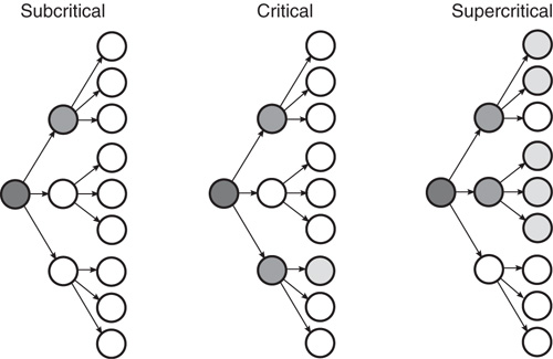
Figure 17.1 Example of subcritical, critical, and supercritical branching processes in which each ancestor produces three offspring who may possess a particular trait (filled circles) or lack it (empty circles). In a critical branching process, each ancestor possessing some trait produces on average one descendant who possesses the trait (center). In a subcritical branching process, each ancestor with the trait produces on average less than one descendant with the trait (left), and in a supercritical branching process, each ancestor with the trait produces on average more than one descendant with the trait (right).
The branching process described above produces a cascade of excitations, henceforth just called an avalanche. Since the avalanche is a stochastic process, that is, the propagation through consecutive generations depends on chance, the duration of an avalanche (number of generations before extinction) will vary according to a distribution determined by the parameters of the process. For example, if each node that is excited at a given generation can produce  excited nodes in the next generation with probabilities
  , the process is critical when these probabilities add exactly to 1 [1, 3–5]. Defining the branching ratio
  to be the expected number of excitations produced by an excited node, the condition for criticality can be written as
Critical branching processes are interesting to theoreticians and experimentalists alike because of their statistical signatures: the probability that an initial excited node results in an avalanche where a total of  nodes are excited in the course of the avalanche is, for large
  , a power law

and the probability that an initial excited node results in a cascade that spans  generations is, for large
  , also a power law

a demonstration of which can be found, for example, in [5]. Remarkably, these exponents are observed in experimental distributions of neuronal avalanches in various settings. The exponent  for the distribution of avalanche sizes has been observed in rat cortical tissue cultures [6–10], awake monkeys [10, 11], and anesthesized mammals [10, 12, 13], while the exponent
  for the distribution of avalanche durations has been observed in resting humans [14]. This suggests that, at the functional level, some aspects of brain activity can be well described by a critical branching process.
The agreement between neuroscience experiments and classical theory of branching processes is surprising given the rather different structure of a neural network compared to a family tree, for example. Indeed, the network of interactions in a classical branching process is always “tree-like” – it has no loops. In contrast, in the cerebral cortex there are recurrent interactions, for example, neuron A can excite neuron B, which can in turn re-excite neuron A. More specifically, various functional brain networks have been reconstructed partially [15–19], and it has been consistently found that these reconstructed networks possess a rich structure, including in some cases a power law distribution in the number of connections per node [15], long-range connections [17], and correlations [19]. Thus, it is imperative to consider the effect that such network structural properties might have on the statistics of avalanche sizes and durations, since they are a key experimental signature of criticality.
The study of propagation of avalanches of activity in complex networks has received considerable attention recently [20–23]. Most of these studies focus on the typical behavior of avalanches in ensembles of networks sharing a certain property (e.g., the degree distribution). In contrast to these previous studies, this chapter describes a theory of avalanche sizes and durations based on [24] which explicitly accounts for networks with complex network topology. This approach allows an analysis of avalanches starting from arbitrary nodes in the network and the effect of nontrivial network structure on the distribution of avalanche sizes and durations. Some of the results presented in this chapter, such as a criterion for criticality based on the largest eigenvalue of an appropriate matrix, have counterparts in the so-called multi-type branching processes [4] if one identifies each individual node with a “particle type.” However, this chapter addresses explicitly the applicability of these results to describe avalanches in complex networks and the effect of modern network topology measures on the distribution of avalanches. Section 17.2 summarizes the terminology and concepts that will be used in subsequent analysis of branching processes in complex networks. Section 17.3 describes how the classical results for the statistics of avalanche durations and sizes mentioned above are affected by the network structure, focusing particularly on the statistics of avalanche durations. Important differences with the classical results include topology-dependent criteria for criticality, and expressions for the distribution of avalanche sizes and durations which explicitly depend on the network topology as described by an appropriate adjacency matrix. In addition, the effect of various network structural properties of interest in modern network research is discussed.
17.2 Description and Properties of Networks
Many common tools have been developed to describe and handle structural aspects of complex networks [25], and their use proves to be instrumental for analyzing the statistics of avalanches in networks. Very generally, a network can be defined as a set of  nodes (or vertices),
  , and a set of
  links (or edges),
  , where each edge is an ordered pair of nodes and the order represents the direction of the link. For example,
  represents a link pointing from node
  to node
  . In the study of neuronal avalanches that follows, each node corresponds to a functional population of neurons.
17.2.1 Network Representation by an Adjacency Matrix
A network with  nodes can be conveniently represented by an
  adjacency matrix
  with entries given by
In many applications, links between different pairs of nodes differ in their importance and/or their effect. For this reason, it is often convenient to relax the definition above to allow any value for each entry of  :
:
The nonzero entries of  are called the link weights, and a network is weighted if not all of the weights are 1. The matrix
  as defined in Eq. (17.5) will be referred to as the adjacency matrix of the network, and the matrix
  as defined in Eq. (17.4) will be referred to as the unweighted adjacency matrix. Undirected networks are represented by a symmetric adjacency matrix satisfying
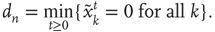
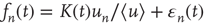
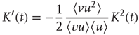
  , where T denotes the transpose matrix. Figure 17.2 illustrates the representation of a small network with an adjacency matrix.
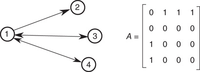
Figure 17.2 Example of an adjacency matrix for a directed network. Each node is indexed by an integer, and the connections from (to) each node are written in the corresponding row (column) of the matrix  .
.
17.2.2 Node Degrees
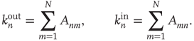
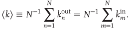
The adjacency matrix contains all the information about the network. However, often one has access only to limited information, such as local information about a sample of nodes or links. One of the properties that can, in absence of all other information, reveal much about the network is the number of incoming and outgoing links per node. In terms of the adjacency matrix, the out-degree and in-degree of node  are
are
When the network is unweighted ( or
or  ), the out- and in-degrees correspond to the number of outgoing and incoming links from and into a node. For weighted networks, the out- and in-degrees generalize this concept and represent the total strength of the outgoing and incoming links. Since every outgoing link from a given node has to be the incoming link of another node, the sum of out-degrees and in-degrees over all nodes must be the same. In fact
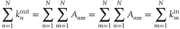
and the mean degree  is defined as
For some networks found in applications, the in- and out-degrees of a given node can be vastly different. For example, the number of hyperlinks pointing to a popular web portal can number in the billions, while the number of hyperlinks pointing to other webpages from that web portal can be of the order of a hundred. Similarly, the directed network of Twitter users (Twitter is a popular microblogging platform) where a link indicates “following” also provides an example with nodes that often have vastly different in-degrees and out-degrees, although in- and out-degrees are still positively correlated in the Twitter network [26].
17.2.3 Degree Distribution
By sampling a large number of nodes from a network, one can estimate the probability that a randomly chosen node has a given in-degree and out-degree, and define the joint degree distribution

In general, the out- and in-degrees are not independent variables. One can still define the marginal distributions
17.10
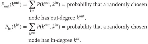
If the out-degree and the in-degree at a given node are independent variables, then
As suggested by the examples mentioned above, the out-degree and in-degree distributions are not necessarily similar. As an example of a network where the out- and in-degree distributions are different, Braha and Bar-Yam studied information-sharing networks, and in particular a pharmaceutical facility development organization [27].
In addition, many real-world networks have degree distributions that are highly heterogeneous. For example, Eguluz et al. [15] observed that functional magnetic resonance imaging (fMRI) networks obtained by imaging human subjects engaged in various tasks have degree distributions that follow approximately a power law, that is,  , where
  represents the in- or out-degree. Networks whose degree distribution follows a power law are often referred to as scale-free networks to indicate the absence of a typical degree, and have been the subject of extensive study in the last decade (see, e.g., [25, 28, 29]). As discussed below, heterogeneous degree distributions result in a different criterion for criticality than the classical result presented in the introduction. Another factor that can modify the classical results degree correlations, described next.
17.2.4 Degree Correlations
Two types of correlations between node degrees are often studied. The first type, node degree correlations, denotes correlations between the out-degree and in-degree at the same node. The presence of node degree correlations implies that knowing information about the in-degree of a randomly chosen node provides some knowledge of its out-degree, and vice versa. Mathematically, it means that the joint degree distribution does not split into a product.
Typically, one is interested not in the full form of the joint degree distribution, but in knowing whether the correlation between out- and in-degrees is positive or negative. If it is positive (negative), nodes with large out-degrees are more likely to have large (small) in-degrees. This can be quantified by the node degree correlation coefficient [30]:
where  denotes an average over nodes. This coefficient is 1 when the out- and in-degrees are independent, is larger than 1 when they are positively correlated, and less than 1 when they are negatively correlated.
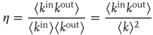
The second type of degree correlation that arises often occurs between the degrees at the ends of a randomly chosen link, referred to as edge degree correlations. In particular, when a link connects nodes  and
and  , a correlation might exist between
  and
and  , between
  and
and  , and so on. Since they have the most effect on network branching processes, this chapter will focus on those between
  and
and  . This can be quantified by the edge degree correlation coefficient [30]:
where  denotes an average over edges,
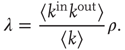
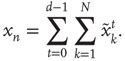
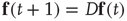
 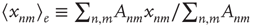 . As with the node degree correlation coefficient, a value of 1 indicates no correlations, and a value larger (smaller) than 1 indicates positive (negative) correlations.1 Figure 17.3 shows examples of the in- and out-degrees of typical nodes and edges in networks with positive and negative correlations: in Figure 17.3a, the in-degrees and out-degrees are negatively correlated. In Figure 17.3b, in-degrees and out-degrees are positively correlated. In Figure 17.3c, the in-degrees and out-degrees coming in and out of two connected nodes are negatively correlated, and in Figure 17.3d they are positively correlated.
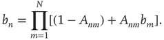
Just like heterogeneity in the degree distributions, node correlations can modify the classical criterion for criticality. They affect the largest eigenvalue of the adjacency matrix, which determines the properties of branching properties on complex networks.

Figure 17.3 Diagram showing examples of the types of links that one might observe in networks with particular  and
and  values. (a) Node in- and out-degree are anticorrelated, (b) node in- and out-degree are correlated, (c) in-degree at node
  is anticorrelated with out-degree at node
  , and (d) in-degree at node
  is correlated with out-degree at node
  .
.
17.2.5 Largest Eigenvalue and the Corresponding Eigenvector
All the properties of networks discussed above, such as the degree distribution and node correlations, are encoded in the network adjacency matrix  . While one can develop analyses of branching processes based only on knowledge of, for example, the degree distribution, the approach of this chapter is to follow [24, 32, 33] and develop an analysis technique based on the adjacency matrix
  . In analyzing the propagation of avalanches in the next sections, repeated matrix–vector multiplications using the matrix
  will arise, and in such cases, the resulting behavior is determined by the eigenvalue of
  with largest magnitude and its corresponding right and left eigenvectors
  and
and  (satisfying
  and
and  ). This eigenvalue and its eigenvectors have a dominant influence on the properties of branching processes in networks, and it is therefore often possible to reduce questions about how network topology affects dynamics on networks to questions about how it affects the dominant eigenvalue
  and its eigenvectors.
The Perron–Frobenius Theorem [34] is fundamental when investigating the largest eigenvalue of network adjacency matrices. It states that an  irreducible, primitive matrix with nonnegative entries has a simple positive eigenvalue
  whose magnitude is larger than the magnitude of all other eigenvalues. Furthermore, its corresponding right and left eigenvectors have positive entries. The criterion of irreducibility, in the context of branching processes in networks, means that an avalanche has a nonzero probability to reach any node when starting from any other node. A matrix
  is primitive if there is an integer
  such that
  . The adjacency matrix of complex networks is typically primitive, and the subsequent analysis here assumes that this condition is satisfied.
While the theoretical results will be stated in terms of the largest eigenvalue  and its eigenvectors
  and
and  , it will be useful to present an approximation to these quantities that allows comparisons with the classical results mentioned in the introduction. When degree correlations are small, the largest eigenvalue and its eigenvectors can be approximated as [30]

17.15

Note that, using the definition of  , Eqs. (17.11) and 17.13 can be rewritten as
One can understand these approximations for  as follows. For random networks without correlations, one has
  and thus
  : that is, the largest eigenvalue represents the average degree (or, if one views the outgoing links from a node as branches, the branching ratio). When there are correlations,
  generalizes the branching ratio, with positive correlations resulting in an effectively larger branching ratio.
17.3 Branching Processes in Complex Networks
This section introduces and analyzes a model of the propagation of avalanches in networks, using many of the descriptive quantities of the previous section. While this section follows [24], for simplicity of exposition only the distribution of avalanche durations is discussed in detail, while similar results for avalanche sizes are summarized.
First, a branching process in a network is defined as follows: Consider a network of  nodes labeled
  . Each node
  has a state
  or
or  . The state
  will be referred to as the resting state and
  as the excited state. At discrete times
  the states of the nodes
  are simultaneously updated as follows: (i) If node
  is in the resting state,
  , it can be excited by an excited node
  ,
,  , with probability
 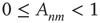 , so that
  . (ii) The nodes that are excited,
  , will deterministically return to the resting state in the next time step,
  . The network of
  nodes is therefore described by an
  weighted network adjacency matrix
  , where
  may be thought of as the strength of the connection from node
  to node
  , and
, and  implies that node
  does not connect to node
  . It will be assumed that, given any two nodes
  and
and  , the probability that an excitation originating at node
  is able to excite node
  (through potentially many intermediate nodes) is not zero. This is equivalent to saying the network is strongly connected, and therefore the matrix
  is irreducible.
The nodes in this network should be thought of as functional units in a coarse-grained description of neuronal activity, where each unit comprises potentially many individual neurons. The probabilities  should be thought of as an effective interaction that aggregates both excitatory and inhibitory connections. Consequently, the effect of modifying the balance of excitation and inhibition (as done experimentally, e.g., in [9]) is represented by a modification of the probabilities
  . These type of coarse-grained branching process models have been used successfully to model various aspects of information processing in neural networks (see [6, 9, 35] and other chapters in this book).
Starting from a single excited node  (
( if
if  and
and  if
if  ), the system is allowed to evolve according to the dynamics above until there are no more excited nodes. The following definitions are introduced to analyze this process: (i) An avalanche is the sequence of excitations produced by a single excited node. (ii) The duration
  of an avalanche is defined as the total number of time steps spanned by the avalanche: if the avalanche starts with
  , then
An avalanche that continues indefinitely is said to have infinite duration. (iii) The size  of an avalanche starting with
  is defined as the total number of nodes excited during an avalanche, allowing nodes to be excited multiple times:
Note that, by this definition, it is possible for an avalanche to have size larger than the total size of the network. The goal is to determine the probability distributions of these variables in terms of the matrix  . For simplicity of exposition, this chapter will be will focused on the distribution of avalanche durations.
Since the interest is specifically in heterogeneous networks, significant differences between different nodes are expected, both in terms of their degree and their location in the network. Therefore, the distribution of avalanche durations for avalanches starting at a specific node  will be studied. To do this, the cumulative distribution of avalanche durations starting at node
  is defined as
Note that the probability distribution of avalanche durations for avalanches starting at node  can be obtained from
  by2
by2
By definition,  is a nondecreasing function of
  which is less than or equal to 1. Therefore, as
  ,
,  must approach a limiting value
  which, from the definition of
  , corresponds to the probability that an avalanche starting at node
  has finite duration:

The behavior of  for large
  will be investigated in order to obtain information about the “tail” of the distribution of avalanche durations (i.e., the behavior of the distribution for large
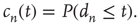
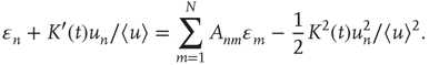
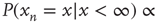
  ). This is illustrated in Figure 17.4. The motivation for this approach stems from experimental results in which the statistics of long (and large) avalanches is claimed to reveal much about the underlying network's critical (or noncritical) state, as discussed in the previous chapters.

Figure 17.4 As a cumulative density function,  is an increasing function of
  . The limiting behavior as
  , that is, how fast
  approaches its limit, reveals information about the tail of the probability distribution of avalanche durations. The limit
  is the probability that an avalanche generated at node
  is finite.
While the presented framework has thus far been applicable to most networks (it has been assumed only that the matrix  is irreducible and primitive), the subsequent analysis will be restricted to a class of networks commonly referred to as locally tree-like networks. These networks have the property that, for most nodes, the nodes that can be reached in a relatively few number of steps form a network that can be approximately described as a tree. To make this more precise, it is assumed that for most nodes
  and relatively small
  , the number of different nodes reachable by paths of length
  or less starting at node
  , which is defined as
  , is close to the total number of paths of length
  or less starting from node
  , which is defined as
  . (Note that, in particular, for
  , this implies that the number of bidirectional edges is small.) Figure 17.5 illustrates this for a particular node in a small network: the number of nodes reachable from the black node by paths of length
  or less (gray nodes) coincides with the total number of paths of length
  or less starting at the black node,
  . In this case, if the expected duration of the avalanches is small, avalanches starting at the dark gray nodes can be approximately treated as independent. Many networks found in applications are locally tree-like [36], and use of the locally tree-like approximation has led to theoretical insights into the behavior of various dynamical processes in networks [32, 37, 38]. Furthermore, use of the locally tree-like approximation has been observed to yield reasonable results even for networks that are not entirely tree-like [36]. Therefore, as a first step toward generalizing the classical results in branching trees to networks, the locally tree-like approximation will be assumed hereafter. It is important to note that, even though the network is assumed to behave locally like a tree, this approximation still captures the effect of factors such as heterogeneous degree distributions and degree correlations.
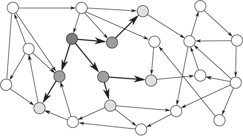
Figure 17.5 The neighborhood of the network around the black node has a tree-like structure.
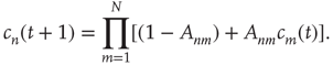
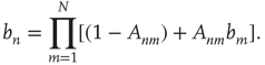
Using the locally tree-like approximation, an equation for  at node
  in terms of the variables
  at other nodes
  can be written down as follows:
The left-hand side is the probability that an avalanche starting at node  lasts less than
  steps. This event is equivalent to the event that for every node
  , either the excitation at node
  does not propagate to node
  (with probability
  ) or it propagates to node
  and the avalanche that is subsequently generated at node
  lasts less than
  steps (with probability
  ). Since the network is assumed to be locally tree-like, avalanches starting at nodes
  are treated as independent events, and thus the right-hand side can be written as the product
As explained above, the behavior of  for large
  , when it is approaching its limiting value
  , is of interest. This limiting value can be obtained by taking the limit
  in Eq. (17.21), and satisfies
The behavior of  as it approaches
  can be analyzed by defining the small distance between
  and its limit
  as
as
Inserting this quantity in Eq. (17.21), one obtains
This expression can be manipulated as follows:
17.28
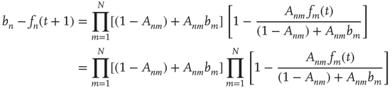
17.30
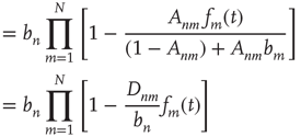
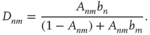
where  is defined as
To determine the behavior when  is large and
 is small, the right-hand side can be expanded in powers of
  keeping only linear terms, to obtain
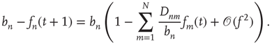
After simplifying, to first order,  satisfies
If an  matrix
  with entries
  and a vector
 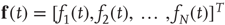 are defined, where the superscript
  denotes the transpose, the previous equation can be written as the vector equation
Starting from some initial time  where
where  is small, and iterating the previous update equation
  times, one has
For large  , the action of the matrix
  on the initial vector results in

where  is the eigenvalue of
  with the largest magnitude, and
  is its corresponding right eigenvector.3 In terms of the quantities
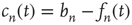 , for large
  they satisfy
where  is the proportionality constant in Eq. (17.36). This analysis is valid as long as
  , since it was assumed that
  decays to zero as
  , and it was found that
  . It turns out that one always has
  . The case
  must be treated separately since this analysis would conclude that
  does not decay to zero (cf. Eq. (17.32)). Inclusion of the second-order terms that were neglected will confirm that
  but as a power law,
  , instead of exponentially. This will be discussed in Section 17.3.3.
17.3.1 Subcritical Regime
In the case  , Eq. (17.37) shows that
  approaches its limit exponentially, reducing the difference to it by a factor of
  in each time step. Using Eq. (17.20), this implies that the probability of an avalanche starting at node
  having duration
  is
is
This result has two components that need to be interpreted: (i) the probability of an avalanche having duration  is proportional to the right eigenvector entry
  of the matrix
  , and (ii) when
  , the probability of an avalanche having duration
  decays exponentially with
  . To understand these results, one needs to determine what
  and
and  represent, and, since the matrix
  is defined in Eq. (17.31) in terms of the entries of
  and of
  , to know what
  is. Recall that
  is the probability that an avalanche starting at node
  has finite duration and satisfies the equation
Note that  for all
  is always a solution of this equation. When
  in Eq. (17.31), the matrix
  reduces to the matrix
  , and therefore
  , where
  is the eigenvalue of
  with largest magnitude discussed in Section 17.2.5. Since the above argument is valid only as long as
  , this suggests that this solution (i.e.,
  ,
,  ,
,  ) will be relevant only when
  . Indeed, it can be shown that this is the only solution when
  (see the Appendices of [24]). Therefore one arrives at the following result: When
  , all avalanches are finite, and for large
  the probability of an avalanche starting at node
  having duration
  is proportional to
  , where
  is the largest eigenvalue of
  and
and  its associated right eigenvector.
This result will now be interpreted and contrasted with the results from uniform branching processes and branching processes on random networks. First, consider the case of networks without correlations, such as random Erd s–Rényi networks, where links are placed with a fixed probability between any pair of nodes [39] (see also [25]). For these networks, as discussed in Section 17.2.5, one can approximate
17.41

Noting that  is the expected number of excited nodes produced by an excitation in node
  , the mean degree
  is equivalent to the average branching ratio
  introduced in Section 17.1. Therefore, for this type of network,
  . The conclusion above then can be interpreted as saying that the distribution of avalanche durations decays exponentially with the rate
  , which agrees with the classical result in critical branching processes in trees [3, 5]. Using the approximation
  , the second part of the result above states that the probability of an avalanche starting at node
  having duration
  is proportional to the out-degree
  of node
  . This is very reasonable since one expects that, everything else being equal, nodes that have more outgoing links (or, more precisely, a larger sum of outgoing weights) should produce longer avalanches.
The results above generalize this intuitive result to more complex network topologies that might have correlations or heterogeneous degree distributions. For example, the largest eigenvalue of a network with a heterogeneous degree distribution, but without degree–degree correlations, can be approximated by (see Eq. (17.16))
The largest eigenvalue  may be interpreted as a generalization of the branching ratio
  , implying that positive node degree correlations will result in a larger effective branching ratio. Since the distribution of avalanche durations decays as
  , positive correlations will result in longer avalanches. In general, various other factors might affect the value of
  , and the advantage of this approach is that the study of the effect of this factor on avalanches is reduced to the study of their effect on
  .
.
For uncorrelated networks, the eigenvector entry  coincides with the local branching ratio
  at node
  . For more general networks, this eigenvector entry can be interpreted as a version of the branching ratio that takes into account both the expected number of nodes that the node
  will generate and the location of these nodes in the network. In general, two nodes
  and
and  that have the same out-degree,
  , and can have very different values of their respective eigenvector entry,
  . As an example, consider the networks shown in Figure 17.6, in which all the nonzero links are assumed to have the same weight:
  if
if  . The network on the left has negative edge–degree correlations (
 ): nodes with many links tend to connect mostly to nodes with few links. On the other hand, the network on the right has positive edge–degree correlations (
 ): nodes with many links tend to connect to each other forming a highly connected core, while poorly connected nodes are in the periphery of the network. These two networks were constructed with the same degree distribution, so that, if one were to calculate the average branching ratio
  , one would obtain
  for both networks. However, the network on the right has a larger eigenvalue
  , and avalanches are more likely to have a longer duration. Intuitively, one can imagine that an avalanche that circulates in the highly connected core will be more likely to have a long duration.
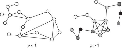
Figure 17.6 Two networks with the same degree distribution but with different edge degree correlations. The network on the left has negative edge degree correlations ( ), while the network on the right has positive edge degree correlations (
 ). The number of nodes reachable in a given number of steps is different if one starts from the black circular node or from the black square node, even though these nodes have same degree. The nodes reachable in one step are colored in dark gray, while the nodes reachable in two steps are colored in light gray. This leads to different statistics of avalanches generated at different nodes, which are captured by the eigenvector entry
  corresponding to a given node.
The networks in Figure 17.6 also serve to illustrate why the distribution of avalanches starting at node  is proportional to the right eigenvector entry
  and not to the out-degree
  . Consider the two nodes marked in black in the network on the right (one circular and the other square), and suppose that they are excited. The circular and square nodes colored in dark gray are those nodes that could be excited in the next time step (with probability
  ) by the black circular and square node, respectively, and the circular and square light gray nodes are the nodes that could be excited after two time steps by the black circular and square node, respectively. While the two black nodes have the same out-degree,
  , the expected size and duration of an avalanche starting at the black circular node should be much larger. The reason is that the eigenvector entry for the black circular node (0.114) is larger than that for the black square node (0.008).
The example above considered a small network, and the description was qualitative. The theory was tested quantitatively by simulating a large number of avalanches on a large network. First, an Erds–Rényi random network [39] was constructed with  nodes by assigning a directed link between any ordered pair of nodes with probability
  . Then, each link was assigned a weight
  uniformly chosen at random from the interval
  . By multiplying the resulting matrix by an appropriate number, a matrix with
  was obtained. Finally, links were rewired so as to decrease the edge–degree correlations (and thus decrease
  ) as follows: two pairs of links
  and
and  are chosen at random, and replaced by two links
  ,
,  only if by doing so the degree–degree correlations become more negative, that is, if
  decreases. By repeating this process multiple times,
  can be decreased to a low enough value and thus a network with negative degree–degree correlations can be constructed (see [30, 31] for more details). Since the resulting network has degree correlations, the approximation
  is no longer valid and the prediction
 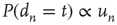 can be verified, and it can be confirmed that, as argued above, it is in general an improvement over using
  .
.
Having constructed a network with degree correlations as described above,  avalanches were simulated, each one starting from a randomly chosen node. For each avalanche, its duration
  and its starting node
  were recorded. Figure 17.7 (from Ref. [24]) shows
  versus
  for a random sample of nodes
  . As can be observed,
  is well predicted by
  , as the points lie approximately on a straight line. On the other hand, using the out-degree
  to predict
  gives bad results: the inset shows a plot of
  versus
  , and it is clear that the correlation between these two variables is significantly smaller.
Figure 17.7 Fraction of avalanches originating at node  that last longer than 30 time steps,
  , versus
  (see text for details about the network used). Theory (Eq. (17.38)) predicts
  . In the inset, the same values
  are plotted against the corresponding out-degree
  . The eigenvector entry
  does a significantly better job than out-degree
  of predicting the duration of avalanches originating at node
  .
.
17.3.2 Supercritical Regime
So far, only the case  , which results in an exponential decay in the duration of avalanches, has been discussed. The analysis of this regime was based on the fact that
  is a solution of Eq. (17.24) toward which
  approaches. When
  , there exists another solution to Eq. (17.24) that satisfies
  (see the Appendices of [24]) and toward which
  converges as
  . Recalling that
  is the probability that an avalanche starting at node
  is finite, a solution
  indicates that there is a positive probability of generating an infinite avalanche. If
  is interpreted as the branching ratio generalized to complex networks, then this conclusion is reasonable: if
  , then, on average, an excited node produces more than one excited node in the next time step and one expects that the number of excited nodes would increase and ultimately saturate. Since
  describes the distribution of finite avalanches, Eq. (17.21) and its analysis still hold. Again, this is valid as long as
  , since in deriving these results it was assumed that
  decays to zero with increasing
  . It can be shown that, if
  , then
  (see the Appendices of [24]). The relationship between
  and
and  is shown graphically in Figure 17.8 from Ref. [24] for an Erds–Rényi random network. Note that when
  ,
,  , so the left half of Figure 17.8 is a straight line with slope 1. While the interpretation of
  in the subcritical regime is clear (i.e.,
  is the effective branching ratio), it is not immediately clear how to interpret
  in the supercritical regime. However, recalling that the distribution of finite avalanches of duration
  decays as
  ,
,  can be interpreted as the effective branching ratio of the finite avalanches. Why does this effective branching ratio decrease even as the actual branching ratio
  increases? As
  increases, finite avalanches have a shorter duration, because long-duration avalanches are more likely to become self-sustained. Therefore, the effective branching ratio of these shorter avalanches is smaller. While this is an intuitive explanation, the mathematical reason is in the derivations above.
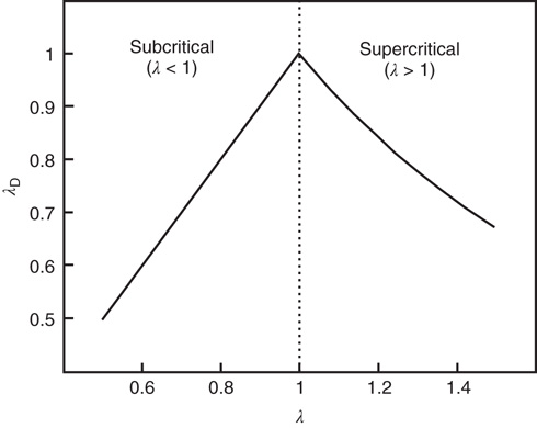
Figure 17.8 Largest eigenvalue of the matrix  with entries in Eq. (17.31),
  , as a function of the largest eigenvalue of the matrix
  ,
,  . The two eigenvalues coincide for
  . The eigenvalue
  can be interpreted as the effective branching ratio of the avalanches that have a finite duration.
Summarizing the results for the supercritical regime, it was found that:
When  , some avalanches have infinite duration, and for large
  the probability of an avalanche starting at node
  having finite duration
  is proportional to
  , where
  is the largest eigenvalue of the matrix
  with entries defined in Eq. (17.31) and
  its associated right eigenvector.
17.3.3 Critical Regime
Of particular interest is the critical regime, in which the distribution of avalanche sizes and durations obeys a power law. So far, the linear analysis of Section 17.3 has been used to analyze the subcritical and supercritical regimes. The linear approach was valid since  , but when
  (and thus
  ), the linear terms that were kept in Eq. (17.32) seem to imply that
  does not grow or decrease with
  (at least for large
  ). However, the terms that were neglected will be sufficient to make
  decrease, albeit at a slower rate. Such behavior is not uncommon in the analysis of the stability of equilibria of nonlinear systems. When a linear stability analysis is inconclusive, the equilibrium is said to be marginally stable and it becomes necessary to determine the stability of the equilibrium by including higher order terms in the analysis. From this standpoint, the previous analysis is a linear stability analysis of the equilibria of the dynamical system defined by the maps Eq. (17.21), and the critical regime corresponds to marginal stability of the equilibrium
  . As explained above, to determine the behavior of
  for large times, it is necessary to keep higher order terms in the expansion of Eq. (17.30), reproduced here for convenience with
  :
:
Since, as a result of the marginal stability, it is expected that  decays to zero at a slower rate than exponentially, it is proposed that the solution
  is given by a function that varies slowly with
  , and that can be extended to continuous values of
  . Under the assumption that
  varies slowly, one can approximate
  by
by
Substituting Eq. (17.44) into Eq. (17.43), one obtains
Assuming  and expanding the product to second order, one obtains, after simplification
The leading order terms as  are
are  on the left-hand side and
  on the right-hand side, so for these to balance it is required that
which is the eigenvector equation  . This means that in this limit
  is proportional to the eigenvector
  of
of  with eigenvalue
  , implying
  , where
  is a proportionality constant. Since
  is independent of time, the constant of proportionality must be time dependent,
  . This argument was made for
  , since the second-order terms were neglected. For finite
  , it is expected that the actual solution of Eq. (17.46) deviates from
 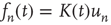 by a small error, so a reasonable ansatz for
  is
is
where  is an error term assumed to satisfy
  and
and  . The term
 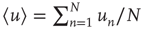 is included to make
  independent of the normalization of
  . Inserting this in Eq. (17.46), neglecting terms of order
  ,
,  , and
, and  , and using the approximation
  (valid when there are many links per node), one obtains
Besides  , which has the desired unknown time dependence, the only unknown in this equation is the error term
  . To eliminate it from the equation, both sides of the equation are multiplied by
  , where
  is the left eigenvector of
  satisfying
  , or
, or 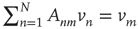 , and summed over
  . The error terms cancel, resulting in an ordinary differential equation (ODE) for
  ,
,
where the notation 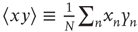 is used. Solving this ODE yields
where  is an integration constant. Using
 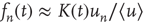 and
and  , one obtains
The probability density function of the duration  , in the continuous time approximation, is given by
  , which evaluates to

For large  ,
,
Therefore, when  , the distribution of avalanche durations for large
  is a power law with exponent
  . As before, the dependence of the distribution on the starting node is through the right eigenvector of
  corresponding to
  . Thus, for the critical regime, it is found that When
  , all avalanches have finite duration, and for large
  the probability of an avalanche starting at node
  having duration
 is proportional to
  , where
  is the largest eigenvalue of matrix
  with entries defined in Eq. (17.31) and
  its associated right eigenvector.
This concludes the analysis of the distribution of avalanche durations. An analysis of the distribution of avalanche sizes can be carried out using similar techniques (see [24]), with the conclusion that the distribution of avalanche sizes for large times is a power law with exponent  when
when  and a power law multiplied by an exponential when
  :
:  , where
  is a parameter that depends on the matrix
  and the vector
 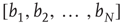 , and is proportional to
  (for details, see [24]). The results for the distribution of avalanche sizes and durations are summarized in Table 17.1.
Table 17.1 Distribution of avalanche durations and sizes.
| Regime | 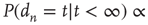 |
 |
 (subcritical) (subcritical) |
 |
 |
 (critical) (critical) |
 |
 |
 (supercritical) (supercritical) |
 |
 |
Table 17.2 Generalization of branching parameters.
| – | Local branching ratio | Global branching ratio |
| Uniform tree |  |
 |
| Unstructured network |  |
 |
| Complex network |  |
 |
The predictions in the table were compared with numerical simulations of avalanches in computer-generated networks. First, heterogeneous networks with  nodes were generated by creating a sequence of
  desired degrees chosen randomly from a power law degree distribution
  and then connecting pairs of nodes at random until the degree of each node reached its desired degree (i.e., the so-called configuration model [25, 29] was used). Then, each nonzero entry in the resulting unweighted adjacency matrix was replaced by a weight chosen uniformly at random from
  . After verifying that the resulting network was irreducible and primitive, its largest eigenvalue was adjusted by multiplying the matrix by a constant, obtaining the matrix
  with largest eigenvalue
  . (This process was used for mathematical convenience, and it is not suggested that brain functional networks adjust their topology in this way. The theory above is independent of how the networks are generated.)
After creating networks as described above with  and
and  , a large number of avalanches were simulated (
 avalanches in the subcritical networks, and
  avalanches in the critical network) and the starting node
  , the duration
  , and the size
  of each avalanche were recorded. Figure 17.9 (from Ref. [24]) shows histograms of the avalanche durations (top panels) and sizes (bottom panels). The symbols indicate the number of avalanches with the duration or size in the horizontal axis, and the dashed lines show the prediction from the theory. Since the predictions above do not specify the proportionality constant, the vertical position in of the dashed curves in the plots is arbitrary. In general, the agreement between the theoretical predictions and the simulations is very good. Additional quantitative comparisons can be done (see [24]) but are not shown here.
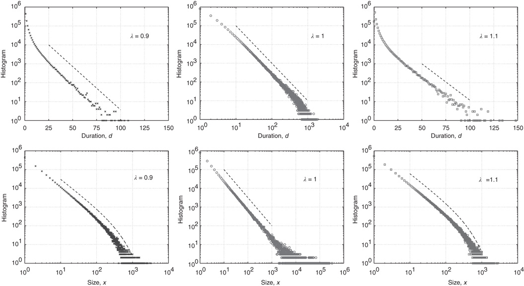
Figure 17.9 Histograms of avalanche durations (top panels) and sizes (bottom panels) for subcritical ( , left panels), critical (
 , middle panels), and supercritical (
 , right panels) networks. The symbols indicate the number of avalanches with the duration or size in the horizontal axis, and the dashed lines show the prediction from the theory (see the table above). The vertical position of the dashed lines is arbitrary.
The bottom panels of Figure 17.9 show that it might be experimentallychallenging to distinguish the distributions of finite avalanche sizes near criticality.These distributions have the form  , where
  is proportional to
  and, therefore, diverges at
  (see [24]). When
  is small enough, the term
  is close to
  and the distribution appears to be a power law with exponent
  . In the examples shown in the figure, the exponential term would not be noticeable if one were to consider only avalanches of size less than
  , and the truncated distributions would appear critical. Only when the full range of observed avalanches is included do the distributions show the effect of the exponential term. While this suggests that it might be hard to pinpoint exactly the critical point in experiments, it also indicates that the regime in which the network is effectively critical, in the sense that its behavior is indistinguishable from the critical state for a wide range of observations, might be relatively large. For observations restricted to avalanches of size less than
  , the effective range of criticality extends approximately from at least
  to
to  . It might be worthwhile to study systematically the robustness of functional aspects such as dynamic range [9, 32, 33, 35] to variations from criticality.
17.4 Discussion
This chapter began with a discussion of critical branching processes in tree-like networks. These processes are characterized by an average branching ratio  which characterizes the nature of the branching process as subcritical, critical, or supercritical if
  ,
,  , or
, or  , respectively. Recent models of avalanche propagation in neural networks [6, 9, 35] have adopted a generalization of the branching ratio which is the average, over all nodes of the network, of the local branching ratio
  , the expected number of nodes that node
  will excite. Thus, the branching ratio
  generalizes to the mean degree
  . In this chapter it was shown that networks with sufficiently complex structure (such as a heterogeneous degree distribution or degree correlations between different nodes) require further generalization. In this case, the local branching ratio at node
  is better approximated by
  , the
, the  th entry in the right eigenvector of the matrix
  . This quantity accounts for the fact that not all nodes are equally effective at propagating excitations in a network with complex topology. It captures not only the expected number of nodes excited by node
  but also how many nodes these will excite in turn, and so on. In short,
  accounts for differences in local network structure. Similarly, the correct generalization of the global branching ratio in this case is given by the largest eigenvalue of the matrix
  ,
,  . This discussion is summarized in the table below.
If the largest eigenvalue  is used in place of
  , the main results from the theory of classical branching processes remain valid, in particular the power law form of the distribution of avalanche sizes and durations at criticality, and also the value of the exponents in the power laws, which have been observed in various experiments of neuronal avalanches [6–13]. In this respect, there does not seem to be a difference between classical branching processes and those in networks. However, it was shown that various network properties can modify the largest eigenvalue and therefore the properties of avalanches of networks. In addition, it is possible to find the statistics of avalanches starting at a particular node, and these statistics can be related to the eigenvector entry of that particular node.
There were some limitations to the theory presented in this chapter. First, it was assumed that the network is locally tree-like. While many networks found in practice can be approximately described as locally tree-like, and a large class of computer-generated networks are also locally tree-like, this approximation might break down when the network has a significant number of short loops, as happens, for example, in networks where nodes are arranged spatially and have a strong local coupling. While it might be possible to extend these results to remove the locally tree-like assumption (which would most certainly modify the criterion for criticality), this is an open problem and left for future research. Another assumption implicit in the theory was that the largest eigenvalue  is well separated from the next largest magnitude of the rest of the eigenvalues. While the theory, as presented above, does not rely on this fact since it was assumed that
  , in practice one observes avalanches up to some large but finite duration. For the approximations to be valid for finite but large
  (in particular, to obtain Eq. (17.32) from Eq. (17.31)) it is required that the separation between
  and the magnitude of the other eigenvalues is not small. This issue has been studied in [40] with the conclusion that this separation is typically very large, except possibly for cases where the network has strong community structure, that is, when it can be divided into groups of nodes such that connections between nodes in the same group are more likely than connections between nodes in different groups. While the analysis in this chapter could perhaps be extended to account for multiple communities, here the simplest case of one community was considered. Finally, the effect of inhibition is typically not included explicitly in branching process models of avalanche propagation, and it was not included in this chapter. It is assumed that decreased inhibition (excitation) results effectively in increased (decreased) probabilities of excitation transmission, and therefore in larger (smaller)
  .
.
The main motivation for the analysis above was to establish a firmer theoretical ground for the observations of criticality in neuronal avalanches in functional brain networks. Typically, the experimentally observed critical exponents are compared with those predicted by branching processes on tree networks. However, it is known that anatomical and functional brain networks often have nontrivial and recurrent structure [15–19]. The analysis presented in this chapter offers an explanation for why the experimentally observed critical exponents match with classical branching process theory predictions in spite of such fundamental differences in the presumed underlying network topology. The analysis extends the class of networks for which one can confidently claim that the observed exponents are predicted theoretically. However, the analysis also offers a warning when interpreting the underlying causes of criticality in brain networks. For example, classical theory would suggest that an experimentally observed change from critical to supercritical dynamics is caused by a change in mean degree in the network. This is potentially misleading; the same change in dynamics could also result from changes in network topology, such as correlations, that leave the mean degree fixed.
Beyond fundamental understanding of existing observations, this chapter offers strategies for controlling avalanche dynamics in complex networks. For example, to prevent large avalanches, disabling the nodes that most contribute to their propagation would be desired. As argued in this chapter, these nodes are those with the largest eigenvector entry  , rather than those with the largest out-degree
  . The two quantities can be very different, and if one used the out-degree to identify the node that produced the longest avalanches in the example used in Figure 17.7, one would identify the wrong node, as the inset shows. Since there has been tremendous progress on the identification and mapping of functional brain networks at various levels [15–19], it is essential to understand the propagation of activity in a network with a specific nontrivial structure. If advances in experimental techniques allow identification of neurons or groups of neurons with large
  , these would likely be good targets to remove when attempting to prevent epileptic seizures. Finally, applications of this work are not restricted to critical brain dynamics, but may include other areas where branching processes in networks occur, such as power grid failure cascades [41] and epidemic propagation on networks [42–44], among others.
A power law distribution of avalanche sizes and durations is perhaps the most distinctive characteristic of critical brain dynamics, but is not the reason for criticality. As in many biological systems, the reason is likely tied to function. Critical dynamics has been observed to result in optimized information processing in neuronal networks [9, 10, 45]. An important example is the maximization of dynamic range at criticality, which was predicted for random networks in [35] and observed experimentally in [9]. Recent work by the authors [32, 33] considered the effect of complex network topology on the dynamic range, and found that, consistent with the results in this chapter, it is maximized when  . As more consequences of critical dynamics for information processing in networks are uncovered, care should be taken to understand the effect of network structure on these processes.
The authors acknowledge useful discussions with Edward Ott, Marshall Carpenter, and Dietmar Plenz. JGR acknowledges support from NSF under Grant No. DMS-0908221. DBL acknowledges support from NSF MCTP Grant No. DMS-0602284, and was also supported by Award Number U54GM088558 from the National Institute Of General Medical Sciences. The content is solely the responsibility of the authors and editors and does not necessarily represent the official views of the National Institute of General Medical Sciences or the National Institutes of Health.
References
- 1. Watson, H. and Galton, F. (1874) On the probability of the extinction of families. J. Anthropol. Inst. Great Br., 4, 138–144.
- 2. Pázsit, I. and Pál, L. (2008) Neutron Fluctuations: A Treatise On the Physics On Branching Processes, Elsevier Science.
- 3. Harris, T. (1963) The Theory of Branching Processes, Springer.
- 4. Athreya, K.B. and Ney, P.E. (1972) Branching Processes, Springer Verlag.
- 5. Zapperi, S., Lauritsen, K., and Stanley, H. (1995) Self-organized branching processes: mean-field theory for avalanches. Phys. Rev. Lett., 75 (22), 4071.
- 6. Beggs, J.M. and Plenz, D. (2003) Neuronal avalanches in neocortical circuits. J. Neurosci., 23 (35), 11–167.
- 7. Beggs, J. and Plenz, D. (2004) Neuronal avalanches are diverse and precise activity patterns that are stable for many hours in cortical slice cultures. J. Neurosci., 24 (22), 5216–5229.
- 8. Stewart, C. and Plenz, D. (2008) Homeostasis of neuronal avalanches during postnatal cortex development in vitro. J. Neurosci. Methods, 169 (2), 405–416.
- 9. Shew, W., Yang, H., Petermann, T., Roy, R., and Plenz, D. (2009) Neuronal avalanches imply maximum dynamic range in cortical networks at criticality. J. Neurosci., 29, 15–595.
- 10. Shew, W., Yang, H., Yu, S., Roy, R., and Plenz, D. (2011) Information capacity and transmission are maximized in balanced cortical networks with neuronal avalanches. J. Neurosci., 31 (1), 55–63.
- 11. Petermann, T., Thiagarajan, T.C., Lebedev, M.A., Nicolelis, M.A.L., Chialvo, D.R., and Plenz, D. (2009) Spontaneous cortical activity in awake monkeys composed of neuronal avalanches. Proc. Natl. Acad. Sci. U.S.A., 106 (37), 15–921.
- 12. Gireesh, E.D. and Plenz, D. (2008) Neuronal avalanches organize as nested theta-and beta/gamma-oscillations during development of cortical layer 2/3. Proc. Natl. Acad. Sci. U.S.A., 105 (21), 7576.
- 13. Hahn, G., Petermann, T., Havenith, M., Yu, S., Singer, W., and Plenz, D. (2010) Neuronal avalanches in spontaneous activity in vivo. J. Neurophysiol., 104 (6), 3312–3322.
- 14. Poil, S.S., van Ooyen, A., and Linkenkaer-Hansen, K. (2008) Avalanche dynamics of human brain oscillations: Relation to critical branching processes and temporal correlations. Human Brain Mapping, 29, 770–777, doi: 10.1002/hbm.20590.
- 15. Eguiluz, V., Chialvo, D., Cecchi, G., Baliki, M., and Apkarian, A. (2005) Scale-free brain functional networks. Phys. Rev. Lett., 94 (1), 18–102.
- 16. Song, S., Sjostrum, P., Reigl, M., Nelson, S., and Chkloskii, D. (2005) Highly nonrandom features of synaptic connectivity in local cortical circuits. Public Library Sci. Biol., 3 (3), 507–519.
- 17. Pajevic, S. and Plenz, D. (2009) Efficient network reconstruction from dynamical cascades identifies small-world topology of neuronal avalanches. PLoS Comput. Biol., 5 (1), e1000–271.
- 18. Wedeen, V.J., Rosene, D.L., Wang, R., Dai, G., Mortazavi, F., Hagmann, P., Kaas, J.H., and Tseng, T.W.Y. (2012) The geometric structure of the brain fiber pathways. Science, 335 (6076), 1628.
- 19. Pajevic, S. and Plenz, D. (2012) The organization of strong links in complex networks. Nat. Phys., 8, 429.
- 20. Samuelsson, B. and Socolar, J. (2006) Exhaustive percolation on random networks. Phys. Rev. E, 74 (3), 036–113.
- 21. Gleeson, J. (2008) Mean size of avalanches on directed random networks with arbitrary degree distributions. Phys. Rev. E, 77 (5), 057–101.
- 22. Benayoun, M., Cowan, J., van Drongelen, W., and Wallace, E. (2010) Avalanches in a stochastic model of spiking neurons. PLoS Comput. Biol., 6 (7), e.
- 23. Hacket, A., Melnik, S., and Gleeson, J. (2011) Cascades on a class of clustered random networks. Phys. Rev. E, 83 (5), 056–107.
- 24. Larremore, D.B., Carpenter, M.Y., Ott, E., and Restrepo, J.G. (2012) Statistical properties of avalanches in networks. Phys. Rev. E Stat. Nonlin. Soft Matter Phys., 85 (6 Pt 2), 066131, arXiv:1204.3861v1.
- 25. Newman, M. (2010) Networks: An Introduction, Oxford University Press.
- 26. Java, A., Song, X., Finin, T., and Tseng, B. (2009) Why we twitter: an analysis of a microblogging community, in Advances in Web Mining and Web Usage Analysis, Lecture Notes in Computer Science, Vol. 5439 (eds H. Zhang, M. Spiliopoulou, B. Mobasher, C. Giles, A.. McCallum, O. Nasraoui, J. Srivastava, and J. Yen) Springer, Berlin / Heidelberg, pp. 118–138, 10.1007/978-3-642-00528-2_7.
- 27. Braha, D. and Bar-Yam, Y. (2004) Topology of large-scale engineering problem-solving networks. Phys. Rev. E, 69, 016–113.
- 28. Albert, R. and Barabási, A. (2002) Statistical mechanics of complex networks. Rev. Mod. Phys., 74 (1), 47.
- 29. Newman, M. (2003b) The structure and function of complex networks. SIAM Rev., 45 (2), 167–256.
- 30. Restrepo, J., Ott, E., and Hunt, B. (2007) Approximating the largest eigenvalue of network adjacency matrices. Phys. Rev. E, 76, 056–119.
- 31. Newman, M. (2003a) Mixing patterns in networks. Phys. Rev. E, 67, 026–126.
- 32. Larremore, D., Shew, W., and Restrepo, J. (2011c) Predicting criticality and dynamic range in complex networks: Effects of topology. Phys. Rev. Lett., 106, 058–101.
- 33. Larremore, D., Shew, W., Ott, E., and Restrepo, J. (2011b) Effects of network topology, transmission delays, and refractoriness on the response of coupled excitable systems to a stochastic stimulus. Chaos, 21, 025–117.
- 34. MacCluer, C. (2000) The many proofs and applications of perron's theorem. SIAM Rev., 42 (3), 487–498.
- 35. Kinouchi, O. and Copelli, M. (2006) Optimal dynamical range of excitable networks at criticality. Nat. Phys., 2, 348–352.
- 36. Melnik, S., Hackett, A., Porter, M., Mucha, P., and Gleeson, J. (2011) The unreasonable effectiveness of tree-based theory for networks with clustering. Phys. Rev. E, 83, 036–112.
- 37. Restrepo, J., Ott, E., and Hunt, B. (2008) Weighted percolation on directed networks. Phys. Rev. Lett., 100, 058–701.
- 38. Ott, E. and Pomerance, A. (2009) Approximating the largest eigenvalue of the modified adjacency matrix of networks with heterogeneous node biases. Phys. Rev. E, 79, 056–111.
- 39. Erds, P. and Gallai, T. (1960) Graphs with prescribed degrees of vertices. Mat. Lapok., 11, 264–274.
- 40. Chauhan, S., Girvan, M., and Ott, E. (2009) Spectral properties of networks with community structure. Phys. Rev. E, 80, 056–114.
- 41. Dobson, I., Carreras, B.A., Lynch, V.E., and Newman, D.E. (2007) Complex systems analysis of series of blackouts: cascading failure, critical points, and self-organization. Chaos, 17, 026–103.
- 42. Pastor-Satorras, R. and Vespignani, A. (2001) Epidemic dynamics and endemic states in complex networks. Phys. Rev. E, 63, 066–117, doi: 10.1103/PhysRevE.63.066117.
- 43. Gomez, S., Arenas, A., Borge-Holthoefer, J., Meloni, S., and Moreno, Y. (2010) Discrete-time markov chain approach to contact-based disease spreading in complex networks. Europhys. Lett., 89, 38–009.
- 44. Allard, A., Noel, P., Dube, L., and Pourbohloul, B. (2009) Heterogeneous bond percolation on multitype networks with an application to epidemic dynamics. Phys. Rev. E, 79 (3), 036–113.
- 45. Yang, H., Shew, W., Roy, R., and Plenz, D. (2012) Maximal variability of phase synchrony in cortical networks with neuronal avalanches. J. Neurosci., 32 (3), 1061–1072.