18
Mechanisms of Self-Organized Criticality in Adaptive Networks

Thilo Gross, Anne-Ly Do, Felix Droste and Christian Meisel

18.1 Introduction

Neural criticality, the hypothesis that the human brain may operate in a critical state, has gained much support over the past decade [1–6]. Previously, a major concern was that reaching criticality would always require the precise tuning of at least one parameter. However starting with the pioneering work of Bornholdt and Rohlf [7], it has become apparent that the self-organization of adaptive networks constitutes a plausible mechanism that could generate and maintain criticality in the brain. In the present chapter, we seek to explain the underlying concepts of adaptive self-organized criticality and build up basic intuition by studying a simple toy model.

18.2 Basic Considerations

In the following, we use the term criticality to denote the behavior that is observed when the system is at a continuous phase transition. We also say that a system at criticality is in a critical state. Statistical physics defines the critical state as a point where the change of an ambient parameter (the control parameter) leads to a nonsmooth response from a property of the system (the order parameter). For phase transitions of second order the nonsmoothness manifests itself as a jump in the first derivative of the order parameter as a function of the control parameter. In other words, in the phase diagram where the order parameter is plotted as a function of a control parameter (see Figure 18.1), the critical point is marked by a sharp corner.

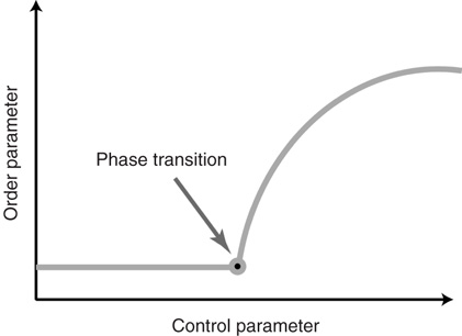
Figure 18.1 Sketch of a continuous phase transition. The critical state is found at the transition point, which appears as a sharp corner in the phase diagram.

As an example, consider, for instance, a sample of neural tissue that is exposed to a drug that alters the excitability of neurons. Here, the concentration of the drug is the control parameter, whereas the overall activity registered in the sample constitutes a suitable order parameter. A second-order phase transition is then characterized by a nonsmooth change of the activity as the drug concentration is varied (e.g., washed out), which is often observed at the onset of activity.

While order and control parameters characterize the system on the macroscopic level, it is conducive for a deeper understanding to consider also the underlying microscopic dynamics. On the microscopic level, a complex system consists of many individual parts (here, neurons and their synapses). For all practical purposes, the number of these parts can be considered to be infinite. Each of the individual units is characterized by its own internal micro-parameters, such as, for instance, conductivities of synapses. The individual units also carry internal micro-variables, such as the membrane voltages of neurons, that change dynamically in time. For connecting the micro and macro levels, note that the control parameter exerts its influence on the system by altering many or all of the micro-parameters, whereas the order parameter appears as a normalized sum over the micro-variables.

In the language of nonlinear dynamics, second-order phase transitions correspond to local bifurcations of a (suitably defined) underlying dynamical system. In contrast to a phase transition, which can be considered a property of the real system, bifurcations are properties of models. Any faithful model of the system under consideration should thus exhibit the same phase transition, whereas the nature of the bifurcation may change depending on how the system is modeled. In particular, a microscopic model of the system will generally exhibit a different bifurcation than a coarse-grained macroscopic model, although both correspond to the same underlying phase transition.

When moving between different scales, the bifurcations that are observed in models cannot change arbitrarily. For instance, an important property of a bifurcation is the codimension. Formally, the codimension of a bifurcation is defined as the number of genericity conditions in the definition of the bifurcation [8]; however, for practical purposes the codimension denotes the number of parameters that have to be changed to find the bifurcation in a typical system. In general, the bifurcations that correspond to phase transitions will be of codimension 1, regardless of the scale of description, which tells us that we need to tune one parameter of the system exactly right to reach the bifurcation point, where the system is critical.

The reasoning presented so far shows that we should not expect criticality to occur accidentally in any given system. Fundamentally, criticality always requires active tuning of one parameter to a precise value. Indeed, this requirement was one of the main concerns that was raised against the criticality hypothesis, as it would seem that criticality required a control circuit that measured the global state (the order parameter) of the brain and adjusted a global control parameter accordingly. The main purpose of the present chapter is to explain why such a global controller is not necessary, and discuss some implications for information processing.

In the following, we propose a basic toy model for criticality, which we subsequently expand in Section 18.4 by a mechanism that drives it robustly to criticality. We then discuss implications for information processing, first in Section 18.5, in the context of the toy model, before generalizing our findings, in Section 18.6, to more realistic neural models.

18.3 A Toy Model

In this section we formulate a toy model that is as easy as possible while containing the ingredients that are needed to build up basic intuition on self-organized criticality in the brain. Most importantly, we need criticality itself, that is, we need a model exhibiting a continuous phase transition. The simplest such system is arguably the epidemiological susceptible-infected-susceptible (SIS) model [9].

This model describes the spreading of an epidemic disease in a population of size . Any given agent is either infected with the disease (state I) or susceptible to the disease (state S). We assume that any given agent encounters other agents at a rate . If the focal agent is infected and the agent encountered is susceptible, then the encountered agent becomes infected with probability . Infected agents recover at a constant rate , and upon recovery immediately become susceptible again.

In the context of the present volume, the reader may want to consider the SIS system as a crude neural model, where the agents are neurons and infected agents represent active (firing) neurons. In this interpretation, the model may seem to be a gross oversimplification neglecting the finite duration of spikes, refractory times, and so on, but, as we show below, it still captures an important essence of neuralcriticality.

Let us start by considering the encounter rate . Even without a detailed analysis, one can guess that the epidemic may go extinct such that no infected agents are left if the encounter rate is sufficiently small. By contrast, the disease can become endemic, infecting a large fraction of the population, if is sufficiently large. Let us now show that the transition between the endemic and the healthy state is a second-order phase transition. To illustrate the points raised in the previous section, we will compute the critical point, the so-called epidemic threshold, in two different ways employing microscopic and macroscopic reasoning, respectively.

We first consider the model on the micro-level. At this level of description, the system consists of a large number of individual agents that change their states in discrete stochastic events. In a sense, considering the whole system at once on this level of detail is too complicated. Thus we have to find a conceptual trick to infer the behavior of the system from the analysis of a small number of agents. For the present system, this can be accomplished by considering a state where there is a small, finite number of infected agents. Since this implies that the density of infected agents vanishes, encounters between infected agents can be neglected and every infected agent can be treated if it were the only infected in an otherwise healthy population. If such an agent causes on average less than one secondary infection before recovering, the disease must eventually go extinct. Although some infected agents may cause more than one secondary infection, the total number of infected in the population will decline exponentially in time. By contrast, if a focal infected agent causes on average more than one secondary infection before recovering, then the number of infected agents will grow exponentially (when infected agents are rare), which is sufficient to guarantee survival of the epidemic.

The average number of secondary infection from a single infected is also known as the basic reproductive number . It can be computed by considering that a typical infected agent will cause secondary infections at the rate until the focal agent itself recovers, which takes in average units of time. Therefore

18.1

From the condition , we can compute the critical encounter rate .

We can thus see that the epidemic will go extinct when and will become endemic when . The critical point thus corresponds to a phase transition between a healthy phase where the dynamics is frozen and a dynamic endemic phase. This microscopic branching ration argument isoften used for detecting critical avalanches of activity in neural tissue and cultures.

A similar result can be obtained by considering the system at the macroscopic level. In this case, we do not consider the states of individual agents but characterize the state of the system by a suitable order parameter. For the epidemic, such an order parameter is the prevalence , which denotes the proportion of infected agents in the population. Given , we know that the total number of infected agents is . Every one of these agents encounters other agents at a rate such that the total rate of encounters of infected agents is . The encountered agent is susceptible with probability and, if susceptible, will be infected with probability . This implies that the total rate at which agents are newly infected is . To translate the gain in numbers back to a gain in prevalence, we divide by and find the gain of prevalence from new infections, . Similarly, we know that given a number of infected agents, , the total rate of recovery will be , which leads to a loss in prevalence of . We can thus write the total change in prevalence as

18.2

We can analyze this differential equation by computing the stationary levels of prevalence, , for which . One can immediately see that this condition is met for such that is a stationary solution; in other words, the healthy state is always stationary. Dividing the right-hand side of the differential equation by , we find the condition for a stationary solution or, equivalently, the nontrivial solution .

Considering the nontrivial solution, we observe that this solution is negative and therefore irrelevant if . For , the second solution corresponds to a finite prevalence of the epidemic and is thus physically relevant. At , both stationary solutions coincide at as the second solution enters the positive space. We thus recover the transition at , which we discovered already by microscopic reasoning. At the macroscopic scale, the transition is marked by an intersection of stationary solution branches, which is known as transcritical bifurcation in dynamical systems theory. In general, such a transition is accompanied by a change in stability of the stationary solutions. Indeed, it can be confirmed by a stability analysis [8] that for the trivial solution is stable, whereas for the trivial solution is unstable and the nontrivial solution is dynamically stable.

Summarizing our findings from the macro-level analysis, we can say that for the system approaches the healthy state, whereas for a small perturbation (i.e., the introduction of some initial infected) is sufficient to drive the system to anendemic state of finite prevalence.

18.4 Mechanisms of Self-Organization

In previous section, we showed by both micro-level and macro-level reasoning that the proposed toy model has a continuous phase transition. Let us now discuss whether and how the toy model has to be extended to self-organize robustly to the critical state associated with this transition. While we will continue to use the epidemiological vocabulary to avoid confusion, this model is now interpreted mainly as a crude model of neural activity.

To enable self-organization to the critical state, at least one of the control parameters must be able to change dynamically in time. For the purpose of illustration, we focus on the parameter . In this section, this parameter becomes a variable that follows its own equation of motion. We then ask under which conditions this equation of motion drives robustly to the critical values . The presentation thus follows a spirit of inverse engineering, where one asks how one would construct a system with given properties, not for the purpose of actual construction but for understanding how the biological system that already has these properties might work. Below, we sometimes say that the agents in the toy model want to organize a critical state. We emphasize that this is done in a physicist's way of speaking and is not meant to imply intentionality of individual neurons or synapses.

The first obstacle that we have to overcome to achieve self-organized criticality is philosophical in nature: Recall that the defining feature of a critical state is the phase transition and therefore the existence of a phase diagram as the one shown in Figure 18.1. However, in order to draw this diagram we must have control over the parameter . If there were some internal dynamics that quickly tuned to the critical value, we would be unable to draw the diagram and hence unable to detect that corresponded to a phase transition. Indeed, deeper analysis reveals that such fast tuning to the critical state would not only obscure the critical nature of the transition point but also would destroy many of its special properties. Roughly speaking, if approaches on the same timescale as the dynamics in the system, it can no longer be considered a tuned parameter but becomes a full-fledged dynamical variable. In the bigger system which now includes this variable, the point is no longer a special transition point but merely the steady-state value of .

For avoiding the problem above, must change on a slower timescale than the internal variables of the system. In this case, the equation governing forms the so-called slow subsystem, in which is still a transition point. In other words, if the dynamics of is sufficiently slow, one can still draw the phase diagram from Figure 18.1 by setting to desired values. We then have sufficient time to observe the value to which settles before changesnoticeably.

The second obstacle that we have to overcome relates to information sensing. The critical value to which we want to tune is not a fundamental constant, but rather depends sensitively on other properties of the systems such as the parameters and in the toy model (cf. Eq. (18.1)). This is a particular concern in biological systems such as the brain, where we need self-organized criticality to work robustly despite ongoing changes to the system in the course of development, aging, and so on. To be able to reach criticality, the system must therefore be able to sense whether the current value of is too low or too high, and adjust it accordingly.

The current hypothesis is that the brain does not have a centralized controller that ensures criticality. Instead, criticality is achieved through synaptic plasticity on every synapse. Such delocalized control implies that at least approximate information about the global state of the brain must be available at every single neuron. The solution to this sensing problem is again timescale separation. The works of Bornholdt and others [7, 10] have shown that this information can be extracted if the local dynamics is observed for a sufficiently long time.

Let us consider the toy model again. In this system, an agent that becomes infected with the disease can tell that the system is in the endemic phase, so (also, for , there might be localized outbreaks; however, these only affect a finite number of agents, a negligible fraction of the system). The agents who become infected thus know that is too high and can thus decisively decrease their personal encounter rate, which on the macro-level leads to a reduction of . By contrast, an agent that is not infected cannot tell whether the whole system is in the healthy phase or she is just lucky while agents elsewhere are infected. If these agents were to increase their personal encounter rate quickly, the system would overshoot the critical point. However, there are two possible strategies that the agents can employ. First, agents could observe their state for a long time; if they do not become infected during this time, it is safe to conclude that the system is in the healthy phase and the encounter rate can be increased. Second, the healthy agents can increase their encounter rates on a slower timescale; then, they would lower it when infected, and thus avoid to overshoot.

Both of the strategies outlined above require a second timescale separation: in the first case, between observing and acting, in the second case between raising and lowering . It has been pointed out that such a timescale separation is always necessary to achieve decentralized self-organized criticality [11]. The first choice, namely observing then acting, is used in many simple models such as in [7]. The second choice, namely decisive decrease, slow increase was used in a simple model in [12] and also occurs naturally in systems that use biologically motivated rules such as spike-timing-dependent plasticity (STDP) [13].

Combining the toy model introduced in Section 18.3 with a suitable plasticity rule following Section 18.4 leads to a system that self-organizesrobustly to a critical state. This is shown explicitly for a related but more realistic neural model in [12].

18.5 Implications for Information Processing

The critical state is optimal for information processing because it can react sensitively to inputs and retain information for a long time. Let us illustrate this again by the example of the toy model. In this model, we can represent internal input by artificially infecting some agents. If , then infecting a small number of agents will only cause a localized outbreak, which disappears exponentially (cf. Eq. (18.2)). If , then there is an ongoing epidemic, but introducing additional infected agents will only have a small and (exponentially) short-lived effect on the ongoing dynamics. By contrast, for , introducing some infected agents can cause a system-level outbreak in an otherwise healthy system. Further, this response decays only geometrically in time and can thus persist for a long time, because of an effect known as critical slowing down .

We note that the nature of a phase transition has direct implication for the code in which information can be fed into the system. In the toy model considered so far, the phase transition can be characterized as a percolation transition where activity starts to spread through the system. Correspondingly, the critical state is sensitive to inputs of activity. In the toy model, we chose to focus on this transition because it is most intuitive. However, for information processing in the brain, other phase transitions such as the synchronization phase transition are probably more relevant.

Our simple toy model cannot sustain synchronized dynamics. But, already somewhat more realistic models of neural dynamics are capable of showing synchronized activity between neurons [13, 14]. If the parameters in such a model are tuned to the synchronization phase transition, which marks the onset of synchronization, then information can be encoded using a synchronization code. Some evidence suggests that the brain is close to both activity [1] and synchronization [2] phase transitions, potentially enabling it to process information using both activity and synchronization codes.

Furthermore, it is interesting to note that the critical state is primarily a resting state. Considering the toy model again, we expect some activity even in absence of external inputs. In the critical state, this activity shows the characteristic power laws that are often used as indicators of criticality [1]. However, subjecting the system to external inputs easily induces large-scale outbreaks and is thus similar to increasing away from the critical state. One would therefore not expect to observe clean power laws during phases of strong information processing.

In the real brain, inputs are never totally absent. We can speculate that the brain compensates for these inputs by tuning to a correspondingly lower value of . In the toy model, this is certainly true because the mechanism of plasticity of the type discussed above would lead to a lower value of . It is thus conceivable that processing inputs slowly detunes the system from criticality and thus impairs further information processing, such that phases of reduced inputs are eventually necessary for retuning the system. This necessity for retuning might be the primary reason for sleep.

18.6 Discussion

In the present chapter, we used a very simple toy model to discuss some properties of plausible mechanisms for self-organized criticality in the brain. Using this model, we were able to gain basic intuition on the requirements and implications of adaptive self-organized criticality. While the real brain and even most models of the brain are much more complex, this basic intuition should remain valid in more complex models. Let us therefore discuss some of the simplifying assumptions that we have made above.

Instead of focusing on a neural model, we discussed a toy model inspired by epidemiology because it allowed an easier representation of some key concepts. While the propagation of the infection in the model can be seen as a crude representation of the propagation of action potentials, it does not include many properties of real neural dynamics, including travel-time delays, refractory times, real-valued action potential, and so on. As a consequence, the toy model is a poor information processor. However, it exhibits the continuous phase transition that we needed for the subsequent discussion of self-organized criticality. The properties of this phase transition do not depend crucially on the underlying model and are therefore independent of the simplifying assumptions.

Furthermore, some idealizations were necessary to draw a clean picture. For instance, we implied that perfect timescale separation is necessary to cleanly define criticality, and a second perfect timescale separation is necessary to reach the critical point precisely. In the real world, the timescale separation between neural dynamics and the relevant mechanisms of synaptic plasticity is certainly large but not infinite. This means that criticality is not reached precisely. However, in practice this is of little consequence. Both the presence of non-negligible noise due to spontaneous activity and the finite number of neurons in the brain imply that the phase transition is not a sharp transition in the real world. In practice, that means that, on close inspection, the phase diagram does not have a sharp corner but a bend with high but finite curvature. In effect, the transition is blurred, becoming a transition region rather then a transition point. While no real system (neural or otherwise) can thus be truly critical, many of the advantageous properties of criticality are found if the system is reasonably close to the transition region.

In summary, we conclude that adaptive self-organized criticality is a plausible mechanism for driving the brain to a critical state where information processing ishighly efficient. In the future, this insight may lead to a deeper understanding of neural dynamics and functioning and could potentially lead to new diagnostic and therapeutic tools. For instance, Meisel et al. [6] have shown that the characteristic power laws associated with neural criticality disappear during epileptic seizures. Furthermore, insights into neural information processing may inspire the design of future computers, which consist of randomly assembled active nano-elements that tune themselves to a critical state where information can be processed.

References

1. 1. Beggs, J.M. and Plenz, D. (2003) Neuronal avalanches in neocortical circuits. J. Neurosci., 23 (35), 11–167.
2. 2. Kitzbichler, M., Smith, M., Christensen, S., and Bullmore, E. (2009) Broadband criticality of human brain network synchronization. PLoS Comput. Biol., 5 (3), e1000–314.
3. 3. Chialvo, D. (2010) Emergent complex neural dynamics. Nat. Phys., 6 (10), 744–750.
4. 4. Expert, P., Lambiotte, R., Chialvo, D., Christensen, K., Jensen, H., Sharp, D., and Turkheimer, F. (2011) Self-similar correlation function in brain resting-state functional magnetic resonance imaging. J. R. Soc. Interface, 8 (57), 472–479.
5. 5. Tetzlaff, C., Okujeni, S., Egert, U., Wörgötter, F., and Butz, M. (2010) Self-organized criticality in developing neuronal networks. PLoS Comput. Biol., 6 (12), e1001–013.
6. 6. Meisel, C., Storch, A., Hallmeyer-Elgner, S., Bullmore, E., and Gross, T. (2012) Failure of adaptive self-organized criticality during epileptic seizure attacks. PLoS Comput. Biol., 8 (1), e1002–312.
7. 7. Bornholdt, S. and Rohlf, T. (2000) Topological evolution of dynamical networks: global criticality from local dynamics. Phys. Rev. Lett., 84, 6114–6117. 10.1103/PhysRevLett.84.6114.
8. 8. Kuznetsov, I. (1998) Elements of Applied Bifurcation Theory, Vol. 112, Springer-Verlag.
9. 9. Anderson, R., May, R., and Anderson, B. (1992) Infectious Diseases of Humans: Dynamics and Control, Vol. 28, Wiley Online Library.
10. 10. Bornholdt, S. and Röhl, T. (2003) Self-organized critical neural networks. Phys. Rev. E, 67 (6), 066–118.
11. 11. Vespignani, A. and Zapperi, S. (1998) How self-organized criticality works: a unified mean-field picture. Phys. Rev. E, 57 (6), 6345.
12. 12. Droste, F., Do, A.-L., and Gross, T. (2013) Analytical investigation of self-organized criticality in neural networks. J. R. Soc. Interface, 78, 20120558.
13. 13. Meisel, C. and Gross, T. (2009) Adaptive self-organization in a realistic neural network model. Phys. Rev. E, 80 (6), 061–917.
14. 14. Levina, A., Herrmann, J.M., and Geisel, T. (2007b) Dynamical synapses causing self-organized criticality in neural networks. Nat. Phys., 3 (12), 857–860.