21
Nonconservative Neuronal Networks During Up-States Self-Organize Near Critical Points

Stefan Mihalas, Daniel Millman, Ramakrishnan Iyer, Alfredo Kirkwood and Ernst Niebur

21.1 Introduction

Criticality refers to the state of a system in which a small perturbation can cause appreciable changes that sweep through the entire system [8]. Self-organized criticality (SOC) means that, from a finite range of initial condition, the system tends to move toward a critical state and stay there without the need for external control of systems parameters [9]. SOC systems are usually slowly driven, steady-state, nonequilibrium systems. Systems exhibiting SOC include models for earthquakes, forest fires, and avalanches of idealized grains toppling down sandpiles [10]. Necessary, but not sufficient, conditions to achieve SOC include (i) partitions of the systems into individual components that interact with each other and with the external environment, (ii) the time scale of internal interactions being much shorter than that of external influences, (iii) individual components/units responding to input only when the input exceeds a given threshold, so that SOC involves the building up of a context-dependent “energy” over long periods followed by transient redistribution of the energy to bring the system back to quiescence, and (iv) the possibility of the system existing in a multitude of metastable states as a result of the threshold.

In a system exhibiting SOC, activity propagates in “avalanche” events in which energy is dissipated intermittently. An avalanche can be characterized by the number of units that become super-threshold as a result of transient internal interactions. For example, an avalanche in a system prone to forest fires caused by lightning wouldconsist of all trees that ultimately burn as a result of a single lightning strike. In a geological context, an avalanche is characterized by the energy released during an earthquake.

The distribution of avalanche sizes in SOC systems follows a power law

21.1

where represents the size of the avalanche and is a scaling exponent which is typically in the range . Power laws are scale-invariant, so for a change in scale by an arbitrary factor

21.2

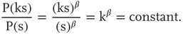
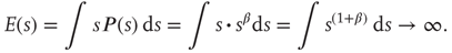
Another way to see this scale invariance is to note that, in the typical range for the critical exponent (), a mean avalanche size does not exist (in an infinite system), that is,

21.3

The branching parameter is a measure of the propagation of excitations in a given network. It is defined as the average number of units that become super-threshold as a result of one unit going above threshold. Perturbations die off quickly for , grow rapidly for , and spread invariably for . Critical systems have [11], while subcritical and supercritical systems have and , respectively.

SOC has been observed in neuronal networks in the form of activity avalanches with a branching parameter near unity and a size distribution that obeys a power law with a critical exponent of about . Neuronal avalanches provide a novel means of characterizing spatiotemporal neuronal activity. By definition, a new avalanche is initiated when a background (external) input is the first input to drive the membrane potential of a neuron above threshold. If however, the membrane potential of a neuron first surpasses threshold as a result of synaptic input from an existing avalanche member, then that neuron is considered a member of the same avalanche. To maintain a common metric for both small and large avalanches, we follow the convention established by Beggs and Plenz [12] and define the branching parameter as the average number of neurons activated directly by the initiating avalanche member (i.e., the second generation of the avalanche).

In nervous systems, the seminal study by Beggs and Plenz [12] demonstrated that adult rat cortical slices and organotypic cultures devoid of sensory input are capable of self-organizing in a critical state. Local field potential (LFP) recordings using multielectrode arrays show activity characterized by brief bursts lasting tens of milliseconds followed by periods of quiescence lasting several seconds. The number of electrodes driven above a threshold during a burst is distributed approximately like a power law. Subsequent experiments in anesthetized rats [13] and in awake monkey cortex [14] have also demonstrated the occurrence of SOC in biological neuronal networks.

Another interesting phenomenon observed during sleep, under anesthesia, and in vitro is the fluctuation of neuronal activity between so-called up- and down-states. These two states are characterized by distinct membrane potentials and spike rates [1–5]. Usually, membrane potential fluctuations around the up-state are of higher order amplitude, whereas the down-state is relatively free of noise.Neurons may exhibit two-state behavior either on account of their intrinsic properties or due to the properties of the network they belong to, or both. At the network level, a high proportion of neurons in large cortical areas alternate between states at the same time [2, 15–18]. While down-states are quiescent [19], up-states have high synaptic and spiking activity [5], resembling that of rapid eye movement (REM) sleep and wakefulness [20]. Differences in synaptic activity and neuronal responsiveness between up- and down-states suggest that the avalanche behavior differs as well.

For a system to maintain criticality, it is typically necessary that the internal state is invariant to perturbations. Neuronal networks endowed with intrinsic homeostatic mechanisms can maintain the critical state [21]. Modeling studies [6] have shown that criticality can be achieved in a conservative network of non-leaky integrate-and-fire neurons with short-term synaptic depression (STSD) [22]. On addition of a voltage leak, however, the networks become nonconservative and require a compensatory current to remain critical. Levina et al. [7] found two stable states, one critical and one subcritical, in a similar conservative network with synaptic depression and facilitation. Nonconservative networks of leaky integrate-and-fire (LIF) neurons also exhibit stable up- and down-states [23], which are obtainable with STSD alone [24].

This chapter, which is an extension of a study by Millman et al. [25], presents results of analytical and numerical investigations of nonconservative networks of LIF neurons with STSD. Analytically, we solve the Fokker–Planck equation for the probability density of the membrane potential in a mean-field approximation. This leads to solutions for the branching parameter in up- and down-states, which is close to unity in the up-state (almost critical behavior) and close to zero (subcritical) in the down-state. Simulated networks of LIF neurons, just as biological neural systems, also exhibit these properties. This behavior persists even as additional biologically realistic features, including small-world connectivity, N-methyl-D-aspartate (NMDA) receptor currents, and inhibition, are introduced. However, in all cases, although the networks get close to the critical point, they never become perfectly critical. We present an additional mechanism, namely finite-width distribution of synaptic weights in a network, that could be tuned along with STSD to obtain a critical state for a nonconservative network.

21.2 Model

The basic model consists of networks of LIF neurons with excitatory synapses and STSD (more general cases will be considered below). Each neuron forms synapses with on average other neurons with uniform probability. Also, each neuron receives Poisson-distributed external input at the rate . Glutamatergic synapticcurrents of the -amino-3-hydroxy-5-methyl-4-isoxazolepropionic (AMPA) type from other neurons, , and external inputs, , are modeled as exponentials with amplitude and integration time constant :

21.4

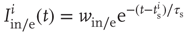
In agreement with physiology, each synapse has multiple () release sites. When a neuron fires spike (at time ), only some sites have a docked “utilizable” vesicle. A utilizable site releases its vesicle with probability , causing a postsynaptic current, Eq. (21.4). To model STSD, is scaled by a site-specific factor , which is zero immediately after a release at site , at time , and recovers exponentially with time constant . Neuronal membranes have potential , resting potential , resistance , and capacitance . Upon reaching the threshold (), the potential resets to after a refractory period . The network dynamics are therefore

21.5

21.6

21.7

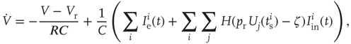
where is a random variable uniformly distributed on , and is the Heaviside step function.

21.2.1 Analytical Solution

To begin with, the time derivative of the mean synaptic utility, 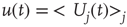, where represents the average over all release sites, can be expressed analytically as

21.8

where is the output firing rate of the network. This can be shown as follows. The time derivative of the mean synaptic utility is the sum of the rate of recovery and the rate of depression, . Recovery happens between vesicle releases, and the average rate can be obtained from the time derivative of Eq. (21.6):

21.9




21.10

to yield the first term on the rhs of Eq. (21.8).

A release site fully depletes following a vesicle release, which happens with probability for each spike, and spikes occur at rate . Thus, the average rate of depletion is

21.11

yielding the second term on the rhs of Eq. (21.8).

The probability distribution of subthreshold membrane potentials, , can be modeled as a drift–diffusion equation [26]. This can be done under the assumption that the correlations between fluctuating parts of the synaptic inputs can be neglected, as shown by Brunel [26]. The drift, with velocity , results from the net change in potential due to synaptic inputs minus the leak. Diffusion arises because synaptic inputs occur with Poisson-like, rather than uniform, timing. The Fokker–Planck equation for the probability density of is

21.12

21.13

21.14

where and are, respectively, the mean changes in membrane potential resulting from a single external and internal input event.

The output firing rate is the probability current that passes through threshold:

21.15

To analyze the fixed points of the dynamical system, the time derivative of can be calculated by numerically evolving the Fokker–Planck equation and used in conjunction with the time derivative of , see Eq. (21.8).

21.2.2 Numerical Evolution of the Fokker–Planck Equation

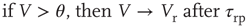
Resetting of the voltage after firing is implemented by boundary conditions that reinsert the probability current through threshold at the resting potential after a refractory period :

21.16

21.17

An initial distribution satisfying the following conditions is first defined:

21.18

21.19

21.20

This initial distribution is taken to be a second-order polynomial

21.21

It is convenient to consider the membrane potential relative to the resting potential.

21.22

The conditions yield the following system of equations for the coefficients of the polynomial:

21.23

21.24

21.25

Solving the system for the coefficients yields

21.26


21.27


21.28

The initial distribution is then evolved according to the partial differential equation (PDE) given by Eqs. (21.12) and (21.14) and the boundary conditions given by Eqs. (21.16) and (21.16), holding and constant. This yields a stationary distribution with a stationary firing rate. Thus we refer to the initial imposed firing rate as and the stationary firing rate as . The value of as a function of is bijective; therefore, a stationary membrane potential distribution can be obtained for any desired stationary firing rate. as a function of can be obtained by evolving the stationary distribution where we use the stationary firing rate as the input firing rate to obtain a self-consistent solution.

At fixed points, (since ). From Eqs. (21.13) and (21.15), we have

21.29

21.2.3 Fixed-Point Analysis

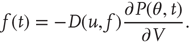
For typical parameter values of cortical neurons [27, 28], the system has two stable fixed points, a quiescent down-state with maximal synaptic utility and an up-state with depressed synaptic utility, separated by a saddle node that sends trajectories to either stable state along the unstable manifold. This is shown in Figure 21.1a.

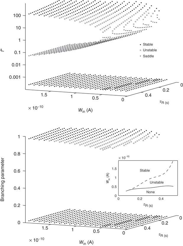
Figure 21.1 Bifurcations of mean-field approximation predict critical up-states and subcritical down-states. (a) Stable fixed points are shown as black, unstable fixed points as hollow dots, and saddle nodes as gray dots. Quiescent stable down-states are ubiquitous in the parameter region shown. When synapses are sufficiently strong and vesicle recovery is sufficiently fast, a stable or unstable high-activity up- state attractor emerges, as well as a saddle node at an intermediate firing rate. (b) Analytical solution for the branching parameter of up- and down-states. Down-states are subcritical with a branching parameter near zero, while the up-states are critical with a branching parameter near unity. Inset: Two-dimensional view of different regions of up-state stability. Parameters: , , , , , , , , , , .

Networks with weak synapses (small ) exhibit only a quiescent down-state ( spikes/s). An unstable up-state and a saddle node emerge with slightly stronger synapses; with even stronger synapses, the up-state becomes stable. Increasing further decreases the firing rate of the saddle node, thereby constricting the basin of attraction for the down-state and making the up-state the dominant feature. When vesicle replenishment is fast (short ), the up-state firing rate is high. As replenishment becomes slower, the up-state firing rate decreases, then the up-state becomes unstable and ultimately collides with the saddle node at a saddle node bifurcation. Beyond the bifurcation, networks do not recover from STSD rapidly enough to sustain up-states.

The branching parameter, that is, the average number of neurons that one neuron is able to activate during an avalanche, is equal to the probability that a postsynaptic neuron's membrane potential will cross threshold due to one input times the number of postsynaptic neurons to which a neuron connects. Since the influence of any given synapse on a cortical neuron is small, the integral can be approximated by the slope near threshold.

21.30

where is the strength of a synapse. This can be expressed in terms of the firing rate at stable states by solving for in Eq. (21.29), using the expression for the u-nullcline (in terms of ) obtained after setting the left hand side of Eq. 21.8 to zero and substituting in Eq. (21.30) to obtain

21.31

The analytical solution shows that (quiescent) down-states are subcritical, while (active) up-states are critical (Figure 21.1b). In down-states, external input dominates the total synaptic input and the branching parameter approaches zero, indicative of subcritical networks. In up-states, input from other neurons within the network dominates synaptic input, the branching parameter approaches unity, and the network is critical.

21.3 Simulations

Networks of neurons described in Eqs. (21.5)–(21.7) were based on a generalized linear LIF model [29] and implemented in an event-driven simulator that is exact to machine precision [30]. Importantly,all computations in this simulation preserve causality, making it possible to trace back the unique spiking event that results in the initiation of an avalanche.

21.3.1 Up- and Down-States

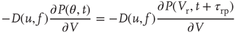
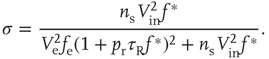
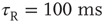
The networks spontaneously alternate between two distinct levels of firing corresponding to up- and down-states (Figure 21.2a). The mean-field approximation models the synaptic inputs that contribute to diffusion and drift as instantaneous steps in the membrane potential. To test whether the mean-field approximation and simulation results converge when synaptic inputs approach steps in the membrane potential, the integration time of the excitatory AMPA currents was decreased to 0.5 ms. In this case, up- and down-state behavior is obtained, but the up-states persist only for tens of milliseconds. Nonetheless, the up-state branching parameter is near unity, the down-state branching parameter is near zero, and the firing rates are in close agreement between simulations and the mean-field approximation, shown in Figure 21.3. Exponential synaptic currents were also modeled with a view to increasing biological realism. Consistent with findings in cortex [31], up- and down-states that persist for simulated seconds are obtained. In agreement with previous findings [2, 23], up-state durations are exponentially distributed (Figure 21.2b). The interspike interval (ISI) distribution during up-states is not exponential (Figure 21.4), leading to the conclusion that spiking during the up-state is not Poisson-distributed.

Figure 21.2 Simulated networks exhibit up- and down-state behavior. (a) Networks spontaneously alternate between a quiescent spiking (down-state) and spikes/s (up- state). (b) The up-state duration distribution is fitted well by an exponential (dashed line, ). (c) At down-to-up transitions, the branching parameter (solid line) increases from zero and overshoots unity before settling near unity; the firing rate (dashed line) likewise overshoots. (d) The branching parameter and firing rate decay toward zero at up-to-down transitions. Same parameters as in Figure 21.1, , ; networks of 300 neurons.

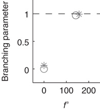
Figure 21.3 Fast excitatory currents approximate instantaneous steps in membrane potential. Firing rate and branching parameter of up- and down-states are in close agreement between mean-field approximation (circles) and simulated networks (stars). Parameters: , , , , , , , , , , , , .

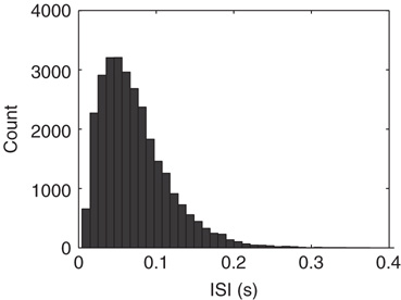
Figure 21.4 Histogram of interspike intervals during the up-state.

21.3.1.1 Up-/Down-State Transitions

The branching parameter follows the firing rate at state transitions. At down-to-up transitions, the branching parameter increases from zero and overshoots unity as activity spreads before finally settling near unity, Figure 21.2c. At up-to-down transitions, the branching parameter decays with the firing rate toward zero, Figure 21.2d.

These transitions can be understood as follows. In the down-state the average synaptic weight (a constant multiple of synaptic utility, u) is near-maximal (Figure 21.5a) while the average synaptic current is near zero, due to near zero firing rate. Conversely, in the up state, the synaptic utility (and hence the average synaptic weight) is low and the firing rate is high (Figure 21.5b). The external inputs have a Poisson distribution, thus having an exponential distribution of the interval between events (Figure 21.6). When external inputs, by chance, sum up to create a large enough event, with strong synaptic weights and large synaptic currents, the system moves for a very brief time in a supercritical regime, which can be observed in Figure 21.2c, as the branching parameter reaches 4 for a very short period. During this supercritical period, the firing rate is very high, resulting in a subsequent decrease in synaptic weight. In these simulations, after a damped oscillation, the system stabilizes in a new regime, the up-state, in which the synapses are weak, but neurons receive, on average, a large synaptic current because of the large stationary firing rate. Thus, external inputs have a larger probability of causing their target neurons to fire than in the down-state, leading to a high rate of avalanches. Each neuron has a probability of almost to cause another neuron to fire (Figure 21.2c), driving the system to criticality. As shown in both the analytical solution and the simulation, the up-state is stable to small perturbations, as a small decrease in the firing rate would cause a compensatory increase in the synaptic weight, and vice versa. However, larger perturbations have the capacity to cause the system to switch to the down-state. An exact prediction of the frequency of the perturbations in the up-state is quite difficult, but it likely does not deviate much from Poisson, as the distribution of the up-state length is well fitted by an exponential (Figure 21.2b).

Figure 21.5 Synaptic utility (gray line) and firing rate (black line) during up-/down-state transitions. (a) At down-/up-state transitions, the synaptic utility is high initially, but decreases upon transition to an up-state. (b) At up-/down-state transitions, the synaptic utility is partially depressed initially, but recovers upon transition to a down- state.

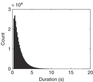
Figure 21.6 The distribution of the duration of down-states. The distribution is fitted well by an exponential with time constant .

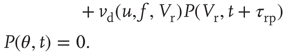
21.3.2 Up-States are Critical; Down-States are Subcritical

Each up- or down-state is composed of hundreds or thousands of avalanches. Avalanche size and lifetime distributions in the up-state follow power laws with critical exponents near and (Figure 21.7a,b; maximum likelihood estimators: and ). Avalanche distributions in the down-state drop off rapidly such that few avalanches of size 10 occur. The method described by Clauset et al. [32] was used to statistically validate criticality. In brief, the maximum likelihood estimators are found under the assumption that avalanche distributions either follow a power law or an exponential. Random power law and exponential distributions are then generated given the maximum likelihood estimators to determine by bootstrap the probability of obtaining a Kolmogorov–Smirnov (KS) distance at least as great as the sample. In all cases, we fail to reject the null hypothesis that avalanche distributions are power-law-distributed (KS-test -values: 0.46 and 0.29 for avalanche size and lifetime, respectively), but we do reject the null hypothesis that the distributions are exponentially distributed ( for avalanche size and lifetime).

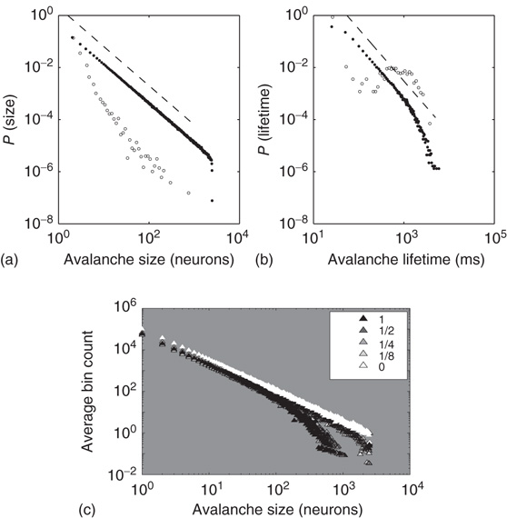
Figure 21.7 Up-states are critical, down-states are subcritical. (a) The frequency distribution of avalanche size (number of neurons) in the up-state (solid dots) follows a power law with slope (dashed line), indicative of critical networks. In the down-state (hollow dots), the distribution is not linear and few avalanches of size occur, indicative of subcritical networks. (b) Similarly, the distribution of avalanche lifetimes follows a power law with slope (dashed line) in the up-state but not the down-state. Same model parameters as Figure 21.2; networks of 2500 neurons. (c) Avalanche size distributions for networks with AMPA and NMDA excitatory currents and different amplitudes of inhibitory currents. The amplitude of inhibitory to excitatory synapses () is given in the legend as a fraction of the excitatory current amplitude. At the highest levels of inhibition, power laws begin to break down near system size. See text for model details.

21.3.3 More Biologically Realistic Networks

The networks can be made more biologically realistic by introducing small-world connectivity, glutamatergic synapses of the NMDA type, and inhibitory currents. While NMDA alone fails to reduce up-state firing rates to biological values, adding inhibition reduces the rates markedly (purely excitatory: 64.0 spikes/s; 1I:8E: 35.6 spikes/s; 1I:4E: 8.7 spikes/s; 1I:2E: 8.7 spikes/s; 1I:1E: 8.4 spikes/s). In all these conditions, up-states are critical and down-states are subcritical, except for the highest levels of inhibition in which the power law in avalanche size distribution begins to break down well before the system size. The models are described in greater detail below.

21.3.3.1 Small-World Connectivity

In networks with small-world connectivity, presynaptic neurons form most synapses with neighboring neurons, and a non-negligible number of connections are made with distant neurons. Figure 21.8 illustrates the connection matrix used to build such networks. The neuronal network is defined as a two-dimensional sheet of neurons. The matrix defines the probability of a synapse forming between any neuron and the neurons around it. The matrix is centered on the presynaptic neuron; note that there is zero probability of the presynaptic neuron forming a connection with itself. There is a 30% probability that the presynaptic neuron will form a connection with any one of the 8 immediately adjacent neuron, a 20% probability for any of the 16 neurons two spaces away, a 10% probability for any of the 24 neurons three spaces away, and a 1% probability for more distant neurons. This type of organization is intended to mimic that of cortical neurons.

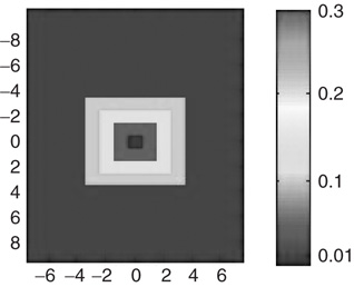
Figure 21.8 Connection matrix for small-world topology.

Networks with small-world connectivity exhibit critical up-states and subcritical down-states (Figure 21.9). Different combinations of recovery time and synaptic strength were used; stronger synapses were used to balance longer recovery times. Parameters: , , , , , , , , , , .

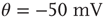
Figure 21.9 Simulation results for small-world networks. Networks with short-term synaptic depression alternate between subcritical down- states and critical up-states for different choices of recovery time and synaptic strength. In all panels, results for three parameter sets are shown, with time constants of 100, 150, and 200 ms, and input of , , and . (a) Sample traces of average firing rates in networks with recovery of synaptic vesicles; results for listed parameter sets from top to bottom. (b) Histograms of firing rates by time bin for all trials. In all cases, most time is spent in a down-state () or an up-state (50–60 Hz). The left-most firing rate in the down-state corresponds to 0 spikes per 100 ms time bin; successive firing rates correspond to additional spikes in a time bin. (c) Avalanche distributions in the down-state; they are indicative of subcritical networks. Distributions are not linear and few avalanches of size occur. The lowest avalanche frequency for networks with each recovery time constant corresponds to one occurrence. (d) Avalanche distributions in the up-state. Network behavior is critical, and power laws show critical exponent near .

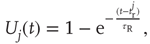
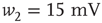
21.3.3.2 NMDA and Inhibition

In the model with NMDA, each synapse is composed of a 20 AMPA:3 NMDA ratio of channels [33]. The pool of NMDA channels include both NR2A (integration time of 150 ms) and NR2B (integration time of 500 ms) in 3 NR2A:1 NR2B ratio. AMPAR (-amino-3-hydroxy-5-methyl-4-isoxazolepropionic receptor) channels have a conductance of 7.2 pS [34] and NMDAR (N-methyl-D-aspartate receptor) channels have a conductance of 45 pS [35], an approximate 1 : 6 ratio in conductance. If all channels are open, this yields a 10 AMPA: 9 NMDA ratio of total conductance. In addition, there is a voltage-dependent magnesium block of NMDAR channels. The proportion of open NMDA channels ranges from 3% to 10% and is given by the following function [36]:

21.32

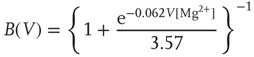
where is in millivolts and [Mg²⁺] is in millimolars (typical value: 1.5 mM).

Since an event-driven simulator is used, conductance-based models cannot be used directly. Instead, the NMDA voltage-dependent conductance is approximated in a current-based model by multiplying the amplitude of the NMDA current by the factor . This factor is updated at each event the neuron experiences (synaptic input or action potential). The simulated networks remain critical in the up-state and subcritical in the down-state with the introduction of NMDA (Figure 21.7c; white triangles).

Inhibition is incorporated in the model by adding 625 inhibitory neurons to the network of 2500 excitatory neurons with AMPA and NMDA channels. Each excitatory neuron sends connections to eight other random excitatory neurons. Inhibitory neurons receive connections from eight random excitatory neurons and send back eight random inhibitory connections. Inhibitory neurons send recurrent connections to eight other random inhibitory neurons. Upon firing, inhibitory neurons induce an exponential current given by Eq. 21.4 in the postsynaptic neuron. Inhibitory (GABAergic) currents have a synaptic time constant of 25 ms, and their amplitude is varied from zero to the same level as excitatory currents. Only excitatory synapses undergo STSD. At the highest levels of inhibition, the avalanche size distribution begins to deviate from a power law only near system size (Figure 21.7c). Parameters are , , , , , , , , , , .

21.3.4 Robustness of Results

Variation of crucial model parameters allows us to inspect the robustness of the results obtained thus far. Whereas the up-state firing rates change only slightly with changes in and (Figure 21.10a), the up-state durations vary widely (Figure 21.10b). In all cases, the branching parameter remains near unity in the up-state and near zero in the down-state (Figure 21.10c), and the up-state critical exponent near (Figure 21.10d).

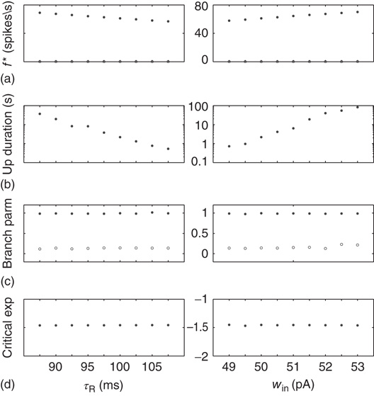
Figure 21.10 Criticality of up-states and subcriticality of down- states are robust to variations of crucial model parameters. (a) Up-state (solid dots) firing rates change slightly as and are changed; down-states (hollow dots) remain quiescent. (b) Up-state durations vary widely with changes in these parameters. (c) Up- and down-state branching parameters remain near unity and zero, respectively, over these parameter regions. (d) The up-state avalanche size critical exponent remains near .

The analytical solution for the branching parameter, given by Eq. (21.31), predicts that networks become subcritical as the external input frequency is increased. Moreover, the system undergoes a saddle-node bifurcation in which the down-state and saddle node collide, leaving only a stable up-state attractor. Figure 21.11 shows how the critical behavior varies during these persistent up-states as a function of the external input rate. As the external input rate is increased, the stationary firing rate does not increase proportionally (Figure 21.11a). In accordance with the mean-field prediction, the branching parameter decreases from unity (Figure 21.11b), while the avalanche size distribution becomes steeper (Figure 21.11c) and no longer follows a power law.

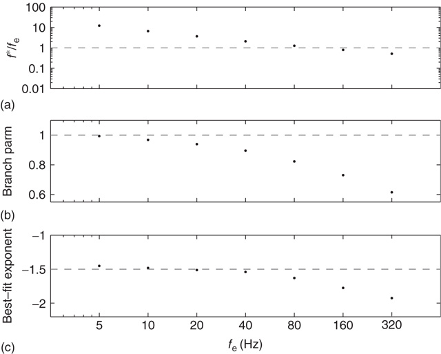
Figure 21.11 Persistent up-states become subcritical with high external input rates. The ratio of stationary firing rate to external input rate decreases with increasing external input rate (a) as does the branching parameter (b) and best fit power law to the avalanche size distribution (c). Same parameters as in Figure 21.2.

Additionally, the robustness of SOC behavior to voltage-dependent membrane resistance can also be investigated. In biological neuronal networks, a neuron's membrane resistance is dependent on its voltage. A voltage-dependent membrane resistance was implemented that resulted in a membrane time constant of 20 ms at rest and 10 ms at threshold, and varying linearly in between. Up-states are critical and down-states are subcritical even with voltage-dependent membrane resistance, as shown in Figure 21.12.

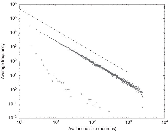
Figure 21.12 Avalanche distributions for simulated networks with voltage-dependent membrane resistance. The avalanche size distribution in the up-state (solid dots) follows a power law with critical exponent near (dashed line), while the distribution in the down- state (hollow dots) does not.

21.4 Heterogeneous Synapses

We have seen thus far that using a specific combination of input firing rate and average synaptic weight makes it possible for a nonconservative network to approach the critical point in the up-state very closely. The addition of STSD makes the up-state an attractor for the network dynamics. As we have seen, avalanches can effectively cause the system to shift from slightly supercritical to slightly subcritical by changing the firing rate of the up-state and the average effective synaptic weight. This causes modest changes in the relative excitability of the neurons participating in an avalanche. There are a number of biological mechanisms, in addition to STSD, that are capable of extending the range over which such excitability changes can be compensated and the system remain in, or very close to, the critical state.

21.4.1 Influence of Synaptic Weight Distributions

So far, we have made the unrealistic assumption that all synapses of a given type have identical strengths. In this section, we explore the presence of synapses that are not necessarily identical but follow a particular distribution. Such distributions of synaptic weights provide an additional compensatory mechanism which can extend the range over which a nonconservative network becomes critical. Numerous experiments have been performed to analyze the distribution of synaptic weights [37–49]. Typically, these experiments show that the distribution of synaptic weights peaks at low amplitudes, resulting in many small-amplitude and a few large-amplitude excitatory postsynaptic potentials (EPSPs) or nhibitory postsynaptic potentials (IPSPs). Distributions have been fitted by lognormal [37], truncated Gaussian [45, 46], or highly skewed non-Gaussian [40, 42, 44, 48] distributions.

The presence of heterogeneous synapses modifies the effects of a localized increase in the firing rate. To repeat, SOC relies on an increase in excitability caused by a raised (closer to threshold) average potential which is compensated by a decrease in excitability due to a decrease in synaptic utility. To understand how heterogeneous synaptic strengths influence this balance in the recurrent networks discussed so far, we looked at a simpler system.

21.4.2 Voltage Distributions for Heterogeneous Synaptic Input

We solve the master equation for a simple network consisting of a homogeneous population of independent and identical LIF neurons with feed-forward excitation [50]. Generalizing the Fokker–Planck approach, the master equation solves for the probability of a neuron to have a voltage in at time .

21.33

with

is the unit step function, and the threshold membrane potential. represents the distribution of synaptic weights, with . and are the minimum and maximum synaptic weights, respectively. represents the sum of all non-synaptic currents, which can be voltage-dependent, but not explicitly time-dependent. For the standard LIF neuron, , where is the membrane time constant.

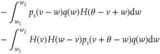
In Eq. (21.33), the first term on the rhs represents the drift due to non-synaptic currents. The second term removes the probability for neurons receiving a synaptic input while at potential . The third term adds the probability that a neuron a distance away in potential receives a synaptic input that changes its potential to . The last term represents a probability current injection of the neuron that previously spiked. It includes the effect of any excess synaptic input above the threshold.

The output firing rate is given by

21.34

The stationary solution of Eq. (21.33) can be obtained as the solution to the following equation:

21.35

where is the stationary probability distribution for the membrane potential.

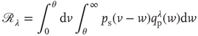
Starting with a stationary state obtained as the solution to Eq. 21.35, with input event rate , the response of the population to fluctuations in input can be quantified by defining

21.36

where is related to the synaptic weight distribution by

21.37

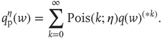
Here, ∗ represents a convolution. represents a Poisson process with mean and events occurring in a time step. By definition, , , , and so on. thus represents the average depolarization of a single neuron, when each neuron in the population receives excitatory inputs on average. If each neuron in the population receives additional inputs on average in the stationary state, then represents the fraction of neurons that spike in the population starting from the stationary distribution . The relative excitability of a neuronal population with a given synaptic weight distribution can then be defined as

21.38

21.4.3 Results for Realistic Synaptic Distributions in the Absence of Recurrence and STSD

We investigated the response to fluctuations for a purely feed-forward “network” of independent LIF neurons, with six different distributions of synaptic weights between and : namely (i) -function (all synapses have the same weight; the case discussed so far), (ii) Gaussian, (iii) exponential, (iv) lognormal, (v) power law with exponent , and (vi) bimodal (a large fraction of synapses have a single small weight and the remaining have a single large weight). The distributions vary in the heaviness of their tails, that is, the fraction of synapses that have weights closer to the threshold . All these distributions have the same mean weight (1 mV), and all networks receive the same input firing rates (500 and 2000 Hz, see below), so that the mean input current is the same. The definitions for the different distributions are asfollows:

1. -function: with .
2. Gaussian: with and .
3. Exponential: with .
4. Lognormal: with and .
5. Bimodal: with , , and .
6. Power law: with and .

The variables , where , are the normalization constants for Gaussian, exponential, and power law distributions, respectively. The corresponding zero-centered second moments are -function (), Gaussian (), exponential (), lognormal (), bimodal (), and power-law ().

The membrane time constant is fixed at . The external input firing rates are chosen as 500 and 2000 Hz. For these choices, for all distributions, the network reaches an equilibrium firing rate approximately equal to that in a down-state for 500 Hz, and to an up-state for 2000 Hz.

For all the six synaptic weight distributions considered, the relative excitability initially rises in both the down-state (Figure 21.13a) and the up-state (Figure 21.14a). Classical definitions of the branching factor in a recurrent network do not apply for our system of independent neurons. But just as in the recurrent network, any fluctuation in this network that increases the average membrane potential carries the potential to produce a spike. Therefore, we use the relative excitability as shown in Figures 21.13a and 21.14a as a simple proxy for the branching factor. Relative excitability is unity for zero added synapses (by definition). In both the up- and down-states, excitability initially increases with added synapses and then decreases. This is consistent with the network becoming first supercritical and, in the cases where excitability falls below unity, it returning to a subcritical state. Note that over the range plotted, for some distributions the excitability does not return to unity or below, but that the range plotted already exceeds what can be expected in physiological situations (for the parameters chosen, activating additional 10 synapses would bring the neuron from rest to nearly the firing threshold). Also note that the decrease of relative excitability below unity for large numbers of added synapses is a compensatory mechanism that is needed to achieve SOC.

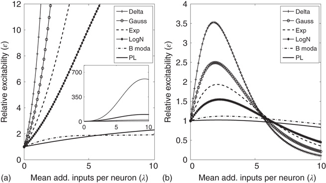
Figure 21.13 Effects of fluctuations in synaptic input due to different synaptic weight distributions in the down-state without (a) and with (b) synaptic depression, respectively. Feed-forward network with 500 Hz external Poisson input for all distributions (Delta: function, Gauss: Gaussian, Exp: exponential, LogN: lognormal, B moda: bimodal, PL: power law). Synaptic weight distributions are matched for mean weight such that drift . The relative excitability initially rises, and the rise is quickest for the distributions that are not heavy-tailed. With STSD, the relative excitability begins to decrease and eventually settles down to values that increase in order of tail-heaviness of the distributions. Note that the excitability remains relatively unchanged for the power law and bimodal distributions. The inset in (a) shows the data at a larger scale on the ordinate which allows us to see the peak of all functions.

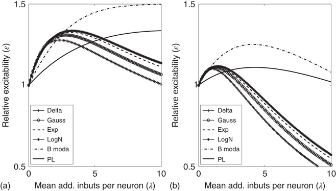
Figure 21.14 Effects of fluctuations in synaptic input due to different synaptic weight distributions in the up-state without (a) and with (b) synaptic depression, respectively. Feed-forward network with 2000 Hz external Poisson input for all distributions (see caption of Figure 21.13 for legend). Synaptic weight distributions are matched for mean weight such that drift . The relative excitability initially rises before it starts to decrease, and the rise is fastest for the distributions that are not heavy-tailed. With STSD, the relative excitability begins to decrease even faster and eventually settles down to values that increase in order of tail-heaviness of the distributions. Note that the excitability remains relatively unchanged for the power law and bimodal distributions.

21.4.4 Heterogeneous Synaptic Distributions in the Presence of Synaptic Depression

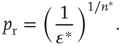
To push the system toward criticality, the rise in excitability can be compensated by introducing STSD. It is implemented by scaling the synaptic utility after each synaptic event, while keeping the distributions unchanged, since all synaptic weights in a distribution are depressed by the same factor. The synaptic utility does not recover and the synaptic utility after an event is decreased by a fraction , which we calculate for each distribution separately, as follows. Let be the number of synapses at which the relative excitability (in the absence of STSD) reaches a peak, and let be the value of this peak. To push the system toward criticality, the strength of the STSD should be such that this peak is close to unity. Therefore, the reduction of synaptic utility should be a factor of

21.39

Intuitively, this choice of ensures that, after extra synapses per neuron are activated on average, the relative excitability in the presence of STSD gets closer to unity.

The relative excitability for the six distributions in the presence of STSD is shown for the down-state in Figure 21.13b and for the up-state in Figure 21.14b. In both states, relative excitability is unity for zero added synapses, then increases to a distribution-dependent peak, after which it falls to a value below unity. For all synaptic distributions, excitability stays closer to unity in the up-state than in the down-state, generalizing our result for the function (Sections 21.2 and 21.3) to all distributions considered. The excursions from unity, both high and low, are most pronounced for the less heavy-tailed distributions. Furthermore, distributions that lack a heavy tail show much larger excursions from unity in the down-state than in the up-state, even in the presence of STSD (Figure 21.13b vs Figure 21.14b). Note that the excitability remains relatively flat around for the networks that are the most influenced by extreme synaptic weights, the power law and bimodal distributions. For these distributions (only), excursions from unity are small in the down-state in the presence of STSD, indicating the possibility of critical behavior not only in the up-state but even in the down-state. In contrast, the largest excursions from unity are shown by the δ-function distribution, which was studied in Sections 21.2 and 21.3. This is the case in both up- and down-states, and both with and without STSD. The lognormal distribution which may be closest to that found in many biological systems [37, 50–55] is in between these extremes.

21.5 Conclusion

The study of complex systems is a vibrant research area and a natural avenue for understanding the behavior of highly nonlinear, densely networked structures like the nervous system. The topic of the present volume is understanding of brain states close to criticality. This state is of particular interest if it is an attractor of the network dynamics, a situation referred to as SOC. Experimental evidence discussed in this and other chapters demonstrate critical behavior in brains and other biological neuronal networks. We have also discussed theoretical work that explains SOC in networks modeled as conservative systems. In many cases, it is, however, more realistic to describe biological neurons as dissipative. We have shown in this chapter that nonconservative neuronal networks can self-organize close to a critical state. This is the case both for simplified neurons and connectivity patterns, as well as when more realism is introduced. However, the complexity of biology usually dwarfs that ofthe better understood physical systems. It is unlikely that the situation in biological systems is as clear-cut as that in a simulated sandpile of idealized grains. If critical behavior is needed for its efficient operation, rather than converging into an ideal state exactly at the critical point, we consider it much more likely that the biological system moves toward criticality without necessarily being pinned exactly in the critical state. It may then stay in its close vicinity, using a variety of mechanisms, some of which we have discussed here. Thus, the system behavior is better characterized as a “bag of tricks” that were acquired during long periods of evolution than by a mathematical abstraction.

Acknowledgment

This work was supported in part by Office of Naval Research, Grant N00141010278, and NIH, Grant R01EY016281.

References

1. 1. Stern, E.A., Kincaid, A.E., and Wilson, C.J. (1997) Spontaneous subthreshold membrane potential fluctuations and action potential variability of rat corticostriatal and striatal neurons in vivo. J. Neurophysiol., 77 (4), 1697.
2. 2. Cossart, R., Aronov, D., and Yuste, R. (2003) Attractor dynamics of network UP states in the neocortex. Nature, 423 (6937), 283–288.
3. 3. Plenz, D., and Kitai, S.T. (1998) Up and down states in striatal medium spiny neurons simultaneously recorded with spontaneous activity in fast-spiking interneurons studied in cortex-striatum-substantia nigra organotypic cultures. J. Neurosci., 18 (1), 266.
4. 4. Steriade, M., Nunez, A., and Amzica, F. (1993) A novel slow () oscillation of neocortical neurons in vivo: depolarizing and hyperpolarizing components. J. Neurosci., 13 (8), 3252.
5. 5. Shu, Y., Hasenstaub, A., Badoual, M., Bal, T., and McCormick, D.A. (2003) Barrages of synaptic activity control the gain and sensitivity of cortical neurons. J. Neurosci., 23 (32), 10–388.
6. 6. Levina, A., Herrmann, J.M., and Geisel, T. (2007b) Dynamical synapses causing self-organized criticality in neural networks. Nat. Phys., 3 (12), 857–860.
7. 7. Levina, A., Herrmann, J.M., and Geisel, T. (2009) Phase transitions towards criticality in a neural system with adaptive interactions. Phys. Rev. Lett., 102 (11), 118–110.
8. 8. Jensen, H.J. (1998) Self-Organized Criticality: Emergent Complex Behavior in Physical and Biological Systems, Cambridge University Press, New York.
9. 9. Bak, P., Tang, C., and Wiesenfeld, K. (1987) Self-organized criticality: an explanation of 1/f noise. Phys. Rev. Lett., 59 (4), 381–384.
10. 10. Bak, P. (1996) How Nature Works: The Science of Self-Organized Criticality, Springer, New York.
11. 11. Christensen, K. and Olami, Z. (1993) Sandpile models with and without an underlying spatial structure. Phys. Rev. E, 48 (5), 3361.
12. 12. Beggs, J.M. and Plenz, D. (2003) Neuronal avalanches in neocortical circuits. J. Neurosci., 23 (35), 11–167.
13. 13. Gireesh, E.D. and Plenz, D. (2008) Neuronal avalanches organize as nested theta-and beta/gamma-oscillations during development of cortical layer 2/3. Proc. Natl. Acad. Sci. U.S.A., 105 (21), 7576.
14. 14. Petermann, T., Thiagarajan, T.C., Lebedev, M.A., Nicolelis, M.A.L., Chialvo, D.R., and Plenz, D. (2009) Spontaneous cortical activity in awake monkeys composed of neuronal avalanches. Proc. Natl. Acad. Sci. U.S.A., 106 (37), 15–921.
15. 15. Lampl, I., Reichova, I., and Ferster, D. (1999) Synchronous embrane potential fluctuations in neurons of the cat visual cortex. Neuron, 22, 361–374.
16. 16. Watson, B.O., MacLean, J.N., and Yuste, R. (2008) UP states protect ongoing cortical activity from thalamic inputs. PLoS One, 3 (12), e3971.
17. 17. MacLean, J.N., Watson, B.O., Aaron, G.B., and Yuste, R. (2005) Internal dynamics determine the cortical response to thalamic stimulation. Neuron, 48 (5), 811–823.
18. 18. Hahn, T.T.G., Sakmann, B., and Mehta, M.R. (2006) Phase-locking of hippocampal interneurons' membrane potential to neocortical up-down states. Nat. Neurosci., 9 (11), 1359–1361.
19. 19. Cowan, R.L. and Wilson, C.J. (1994) Spontaneous firing patterns and axonal projections of single corticostriatal neurons in the rat medial agranular cortex. J. Neurophysiol., 71 (1), 17.
20. 20. Destexhe, A., Hughes, S.W., Rudolph, M., and Crunelli, V. (2007) Are corticothalamic Up states fragments of wakefulness? Trends Neurosci., 30 (7), 334–342.
21. 21. Hsu, D. and Beggs, J.M. (2006) Neuronal avalanches and criticality: a dynamical model for homeostasis. Neurocomputing, 69 (10), 1134–1136.
22. 22. Markram, H., Lübke, J., Frotscher, M., and Sakmann, B. (1997a) Regulation of synaptic efficacy by coincidence of postsynaptic APs and EPSPs. Science, 275, 213–215.
23. 23. Parga, N. and Abbott, L.F. (2007) Network model of spontaneous activity exhibiting synchronous transitions between up and down states. Front. Neurosci., 1 (1), 57.
24. 24. Holcman, D. and Tsodyks, M. (2006) The emergence of up and down states in cortical networks. PLoS Comput. Biol., 2 (3), e23.
25. 25. Millman, D., Mihalas, S., Kirkwood, A., and Niebur, E. (2010) Self-organized criticality occurs in non-conservative neuronal networks during Up states. Nat. Phys., 6 (10), 801–805.
26. 26. Brunel, N. (2000) Dynamics of sparsely connected networks of excitatory and inhibitory spiking neurons. J. Comput. Neurosci., 8 (3), 183–208.
27. 27. Südhof, T.C. (2004) The synaptic vesicle cycle. Annu. Rev. Neurosci., 27, 509.
28. 28. Dobrunz, L.E. and Stevens, C.F. (1997) Heterogeneity of release probability, facilitation, and depletion at central synapses. Neuron, 18 (6), 995–1008.
29. 29. Mihalas, S. and Niebur, E. (2009) A generalized linear integrate-and-fire neural model produces diverse spiking behavior. Neural Comput., 21 (3), 704–718.
30. 30. Mihalas, S., Dong, Y., von der Heydt, R., and Niebur, E. (2011) Event-related simulation of neural processing in complex visual scenes. 45th Annual Conference on Information Sciences and Systems IEEE-CISS-2011, IEEE Information Theory Society, Baltimore, MD, 1–6.
31. 31. Amzica, F. and Steriade, M. (1995) Short-and long-range neuronal synchronization of the slow () cortical oscillation. J. Neurophysiol., 73 (1), 20.
32. 32. Clauset, A., Shalizi, C.R., and Newman, M.E. (2009) Power-law distributions in empirical data. SIAM Rev., 51 (4), 661–703.
33. 33. Franks, K.M., Bartol, T.M., and Sejnowski, T.J. (2002) A Monte Carlo model reveals independent signaling at central glutamatergic synapses. Biophys. J., 83 (5), 2333–2348.
34. 34. Jonas, P. and Sakmann, B. (1992) Glutamate receptor channels in isolated patches from CA1 and CA3 pyramidal cells of rat hippocampal slices. J. Physiol., 455 (1), 143–171.
35. 35. Keller, D.X., Franks, K.M., Bartol, T.M., and Sejnowski, T.J. (2008) Calmodulin activation by calcium transients in the postsynaptic density of dendritic spines. PLoS One, 3 (4), e2045.
36. 36. Jahr, C. and Stevens, C. (1990) Voltage dependence of NMDA-activated macroscopic conductances predicted by single-channel kinetics. J. Neurosci., 10, 3178–3182.
37. 37. Song, S., Sjostrum, P., Reigl, M., Nelson, S., and Chkloskii, D. (2005) Highly nonrandom features of synaptic connectivity in local cortical circuits. Public Lib. Sci. Biol., 3 (3), 507–519.
38. 38. Sjöström, P.J., Turrigiano, G.G., and Nelson, S.B. (2001) Rate, timing, and cooperativity jointly determine cortical synaptic plasticity. Neuron, 32 (6), 1149–1164.
39. 39. Mason, A., Nicoll, A., and Stratford, K. (1991) Synaptic transmission between individual neurons of the rat visual cortex in vitro. J. Neurosci., 11, 72–84.
40. 40. Lefort, S., Tomm, C., Floyd Sarria, J., and Petersen, C.C. (2009) The excitatory neuronal network of the C2 barrel column in mouse primary somatosensory cortex. Neuron, 61 (2), 301.
41. 41. Frick, A., Feldmeyer, D., Helmstaedter, M., and Sakmann, B. (2008) Monosynaptic connections between pairs of L5A pyramidal neurons in columns of juvenile rat somatosensory cortex. Cereb. Cortex, 18 (2), 397–406.
42. 42. Markram, H., Lübke, J., Frotscher, M., Roth, A., and Sakmann, B. (1997b) Physiology and anatomy of synaptic connections between thick tufted pyramidal neurones in the developing rat neocortex. J. Physiol., 500 (Pt 2), 409.
43. 43. Sayer, R., Friedlander, M., and Redman, S. (1990) The time course and amplitude of epsps evoked at synapses between pairs of CA3/CA1 neurons in the hippocampal slice. J. Neurosci., 10 (3), 826–836.
44. 44. Feldmeyer, D., Egger, V., Lübke, J., and Sakmann, B. (1999) Reliable synaptic connections between pairs of excitatory layer 4 neurones within a single ‘barrel’ of developing rat somatosensory cortex. J. Physiol., 521 (1), 169–190.
45. 45. Isope, P. and Barbour, B. (2002) Properties of unitary granule cell Purkinje cell synapses in adult rat cerebellar slices. J. Neurosci., 22 (22), 9668–9678.
46. 46. Brunel, N., Hakim, V., Isope, P., Nadal, J.P., and Barbour, B. (2004) Optimal information storage and the distribution of synaptic weights: perceptron versus Purkinje cell. Neuron, 43 (5), 745–757.
47. 47. Ikegaya, Y., Sasaki, T., Ishikawa, D., Honma, N., Tao, K., Takahashi, N., Minamisawa, G., Ujita, S., and Matsuki, N. (2013) Interpyramid spike transmission stabilizes the sparseness of recurrent network activity. Cereb. Cortex, 23 (2), 293–304.
48. 48. Miles, R. (1990) Variation in strength of inhibitory synapses in the CA3 region of guinea-pig hippocampus in vitro. J. Physiol., 431 (1), 659–676.
49. 49. Holmgren, C., Harkany, T., Svennenfors, B., and Zilberter, Y. (2003) Pyramidal cell communication within local networks in layer 2/3 of rat neocortex. J. Physiol., 551 (1), 139–153.
50. 50. Iyer, R., Menon, V., Buice, M., Koch, C. and Mihalas, S. (2013) The Influence of Synaptic Weight Distribution on Neuronal Population Dynamics. PLoS Comput Biol, 9 (10), e1003248. doi:10.1371/journal.pcbi.1003248.
51. 51. Beyer, H., Schmidt, J., Hinrichs, O., and Schmolke, D. (1975) A statistical study of the interspike-interval distribution of cortical neurons. Acta Biol. Med. Ger., 34 (3), 409.
52. 52. Burns, B. and Webb, A. (1976) The spontaneous activity of neurones in the cat's cerebral cortex. Proc. R. Soc. London. Ser. B Biol. Sci., 194 (1115), 211–223.
53. 53. Webb, A. (1976a) The effects of changing levels of arousal on the spontaneous activity of cortical neurones. I. Sleep and wakefulness. Proc. R. Soc. London. Ser. B Biol. Sci., 194 (1115), 225–237.
54. 54. Webb, A. (1976b) The effects of changing levels of arousal on the spontaneous activity of cortical neurones. II. Relaxation and alarm. Proc. R. Soc. London. Ser. B Biol. Sci., 194 (1115), 239–251.
55. 55. Levine, M. (1991) The distribution of the intervals between neural impulses in the maintained discharges of retinal ganglion cells. Biol. Cybern., 65, 459–467.
56. 56. Bershadskii, A., Dremencov, E., Fukayama, D., and Yadid, G. (2001) Probabilistic properties of neuron spiking time-series obtained in vivo. Eur. Phys. J. B, 24 (3), 409–413.