22
Self-Organized Criticality and Near-Criticality in Neural Networks

Jack D. Cowan, Jeremy Neuman and Wim van Drongelen

We show that an array of -patches will self-organize around critical points of the directed percolation phase transition and, when driven by a weak stimulus, will oscillate between UP and DOWN states, each of which generates avalanches consistent with directed percolation. The array therefore exhibits self-organized criticality (SOC) and replicates the behavior of the original sandpile model of [1]. We also show that an array of patches will also self-organize to a weakly stable node located near the critical point of a directed percolation phase transition, so that fluctuations about the weakly stable node will also follow a power slope with a slope characteristic of directed percolation. We refer to this as self-organized near-criticality (SONC).

22.1 Introduction

Ideas about criticality in nonequilibrium dynamical systems have been around for at least 50 years or more. Criticality refers to the fact that nonlinear dynamical systems can have local equilibria that are marginally stable, so that small perturbations can drive the system away from the local equilibria toward one of several locally stable equilibria. In physical systems, such marginally stable states manifest in several ways; in particular, if the system is spatially as well as temporally organized, then long-range correlations in both space and time can occur, and the statistics of the accompanying fluctuating activity becomes non-Gaussian, and in fact is self-similar in its structure, and therefore follows a power law. Bak et al. [1] introduced a mechanism whereby such a dynamical system could self-organize to a marginally stable critical point, which they called self-organized criticality. Their paper immediately triggered an avalanche of papers on the topic, not the least of which was a connection with or scale-free noise. However, it was not until another paper appeared, by Gil and Sornette [2], which greatly clarified the dynamical prerequisites for achieving SOC, that a real understanding developed of the essential requirements for SOC: (i) an order-parameter equation for a dynamical systemwith a time-constant , with stable states separated by a threshold; (ii) a control-parameter equation with a time-constant ; and (iii) a steady driving force. In Bak et al.'s classic example, the sandpile model, the order parameter is the rate of flow of sand grains down a sandpile, the control parameter is the sandpile's slope, and the driving force is a steady flow of grains of sand onto the top of the pile. Gil and Sornette showed that, if , then the resulting avalanches of sand down the pile would have a scale-free distribution, whereas if , then the distribution would also exhibit one or more large avalanches.

In this chapter, we analyze two neural network models. The first is in one-to-one correspondence with the Gil–Sornette SOC model, and therefore also exhibits SOC. The second is more complex and, instead of SOC, it self-organizes to a weakly stable local equilibrium near a marginally stable critical point. We therefore refer to this mechanism as self-organized near-criticality, or SONC.

22.1.1 Neural Network Dynamics

Consider first the mathematical representation of the dynamics of a neocortical slab comprising a single spatially homogeneous network of excitatory neurons. Such neurons make transitions from a quiescent state to an activated state at the rate and back again to the quiescent state at the rate , as shown in Figure 22.1.

Figure 22.1 Neural state transitions. is the activated state of a neuron, is the inactivated or quiescent state, and is a constant, but depends on the number of activated neurons connected to the th neuron and on an external stimulus .

It is straightforward to write down a master equation describing the evolution of the probability distribution of neural activity in such a network. We consider active excitatory neurons, each becoming inactive at the rate . This causes a flow of rate out of the state proportional to , hence a term . Similarly, the flow into from , caused by one of active excitatory neurons becoming inactive at rate , gives a term . The net effect is a contribution

22.1

In state , there are quiescent excitatory neurons, each prepared to spike at the rate , leading to a term , where the total input is , and is the function shown in Figure 22.2.

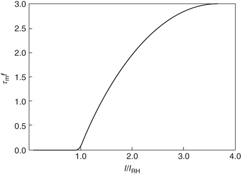
Figure 22.2 Graph of the firing rate function . is the membrane time constant (in milliseconds.). is the input current, where is the threshold or rheobase current.

Correspondingly, the flow into the state from due to excitatory spikes is given by . The total contribution from excitatory spikes is then

22.2

Putting all this together, the probability evolves according to the master equation

22.3

Using standard methods, it is easy to derive an equation for the evolution of the average number of active neurons in the network. The resulting equation takes the form

22.4

where , and is the simplest form of the Wilson–Cowan equations, [3]. This mean-field equation can be obtained in several ways: in particular, it can be obtained using the van Kampen “system-size expansion” of the master equation about a locally stable equilibrium or fixed point of the dynamics, [4]. However, such an expansion breaks down at a marginally stable fixed point, which is the situation to be analyzed in this chapter, and a different method must be used to analyze such a situation.

Before proceeding further, we note that it is straightforward to extend these equations to deal with spatial effects. In such a case, the variable is extended to which represents the density of active neurons at the location at time , and the total input becomes the current density

22.5

22.1.2 Stochastic Effects Near a Critical Point

To deal with the effects of fluctuations near criticality, we use the methods of statistical field theory. Essentially, we rewrite the solution of the spatial master equation in the form of a Wiener path integral. We then apply the renormalization group method [5] to calculate the statistical dynamics of the network at the marginally stable or critical points. The details of this procedure can be found in [6]. The main result is that the random fluctuations about such a critical point have the statistical signature of a certain kind of percolation process on a discrete lattice, called directed percolation. Such a random process is similar to isotropic percolation that occurs in the random formation of chemical bonds, except that there is a direction – in the neural network case a time direction – to the process. The statistical signature of directed percolation occurs in a large class of systems, and is independent of their various dynamical details, and is therefore taken to define a universality class. It is found in random contact processes, branching and annihilating random walks, predator–prey interactions in population dynamics [7], and even in bacterial colonies growing in Petri dishes [8]. Thus stochastic neural networks described by the simple Markov process we depicted in Figure 22.1 exhibit a nonequilibrium phase transition whose statistical signature is that of directed percolation [9].

In what follows, we describe how these methods and results can be used to provide insights into the nature of fluctuating neural activity found in functional magnetic resonance imaging (fMRI), electroencephalography (EEG), and local field potentials (LFPs) both in cortical slices and slabs and in the intact neocortex.

22.2 A Neural Network Exhibiting Self-Organized Criticality

We first consider a simple network comprising only excitatory neurons which exhibits SOC. We start by considering the network module shown in Figure 22.3.

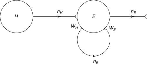
Figure 22.3 A recurrent excitatory network driven by the input , acting through the synaptic weight .

Note that this network is also spatially organized. We consider the overall system to have the geometry of a two-dimensional sheet, so that each homogeneous patch is coupled to four neighboring patches. The local dynamics of each patch is bistable. There is a stable resting state for small values of , and a nonzero stable state N.

We now assume that the synaptic weight is modifiable and anti-Hebbian, and makes transitions from a state to a potentiated state at the rate and back again (synaptic depression) at the rate , as shown in Figure 22.4

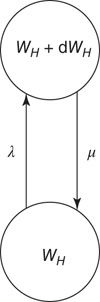
Figure 22.4 Synaptic weight transitions. Transitions from the synaptic weight to occur at the rate , and the return transition at the rate .

Such a Markov process satisfies the master equation

22.6

where

22.7

and

22.8

The resulting mean-field equation takes the form

22.9

or

22.10

In the continuum limit, Eq. 22.10 becomes

22.11

where is the rate constant for weight changes, is the density of synapses at , and is the state-dependent function

22.12

where , is a constant neural activity, and is a constant derived from the window function of spike-time-dependent plasticity (STDP) used in [10]. The ratios , , and are zero dimensional, and represent the mean numbers of spikes.

In Eqs. 22.10 and 22.11, the synaptic weight is depressed if the postsynaptic cell fires and potentiated if it does not. This is an anti-Hebbian excitatory synapse. Such an equation type was first introduced by Vogels et al. [10] for a purely feed-forward circuit with no loops, and a linear firing rate function , in which the synapse was inhibitory rather than excitatory, and Hebbian rather than anti-Hebbian. The Vogels formulation has an important property: the equation can be shown to implement gradient descent to find the minimum of an energy function, the effect of which is to balance incoming excitatory and inhibitory currents to the output neuron. Equation 22.10 is an extension of the Vogels equation to the case of circuits with feedback loops, and a nonlinear firing rate function , and incorporates modifiable synapses which are excitatory and anti-Hebbian. In fact, there is experimental evidence to support such synapses [11].

22.2.1 A Simulation of the Combined Mean-Field Equations

The combined effect of the mean-field Eqs. 22.4 and 22.10 can be easily computed. The results are shown in Figure 22.5.

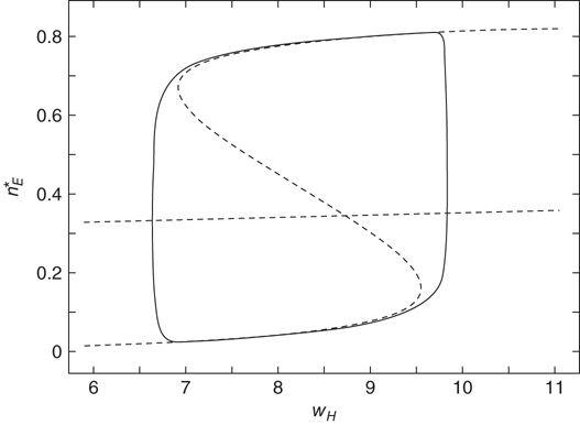
Figure 22.5 Neural state transitions between a ground state and an excited state. Parameter values: . is the fixed-point value of , and is the magnitude of the anti-Hebbian synapse in the input path. The fast excitatory nullcline is shown as the dark grey dashed line, and the slow inhibitory nullcline as the light dashed line.

It will be seen that, for low values of , the synaptic weight is potentiated until the fixed point reaches a critical point (a saddle–node bifurcation), at which point the network dynamics switches to a new fixed point with a high value of . But then the anti-Hebbian term in the dynamics kicks in, and depresses until again becomes unstable at the upper critical point (another saddle–node bifurcation) and switches back to the lower fixed-point regime, following which the cycle starts over. This is therefore a hysteresis cycle, and is an exact representation of the dynamics of the sandpile model.

22.2.2 A Simulation of the Combined Markov Processes

The simulation above provides us with an outline of the general dynamical behavior of the coupled mean-field equations, but it provides no information about the system dynamics beyond the mean-field region. But here we can make use of the Gillespie algorithm for simulating the behavior of Markov processes in which the underlying mean-field dynamics is stable [12]. We therefore simulated the behavior of the two Markov processes introduced earlier, in which the first process describes the stochastic evolution of the firing rate , driven by a weak input coupled to the -system by the modifiable anti-Hebbian weight , and the second process describes the evolution of driven by both the external stimulus and the network variable .

The network we simulated is two dimensional, and comprises neurons with nearest neighbor connections and periodic boundary conditions, in which each neuron receives current pulses from all four nearest neighbors, and also from an external cell via the synapse . The simulations are shown in Figure 22.6.

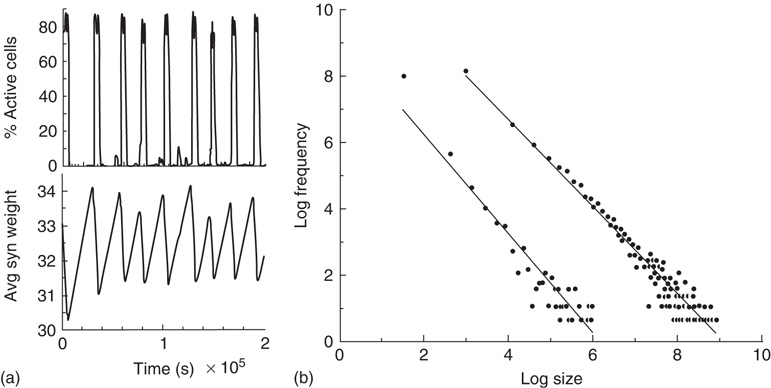
Figure 22.6 Neural state transitions between a ground state and an excited state in a two-dimensional network of excitatory neurons with nearest neighbor connections. (a) Population activity and mean synaptic weight versus time. Activity levels display cyclic behavior with “UP” and “DOWN” states. (b) Avalanche distribution of DOWN states (black dots) and UP states (black dots). Parameter values: , , and . is the function introduced in Figure 22.2.

The reader is referred to [6] for all the details. However, it will be seen that the neural population behavior shown in Figure 22.6a is consistent with that shown in Figure 22.5, and the changes in are also consistent with the changes shown in that figure. Figure 22.6b however, shows the burst or avalanche-size distribution of the underlying population spiking activity. Note that the fluctuations in spiking activity about the lower nullcline, or DOWN state, have a power law distribution with a slope of about , whereas those about the higher nullcline or UP state also show a power law distribution with a slope of about −1.3.

However, the results described above differ in certain respects from those obtained by Gil and Sornette [2]. In their simulations, they used time constants corresponding to and . Both simulations produced similar power laws for small avalanche sizes, but using the larger time constant also generated isolated large system-size avalanches, orders of magnitude greater than the smaller avalanches. In our simulations, the ratio used was . The results we found are that there are two branches of power-law-distributed avalanches, corresponding to the UP and DOWN mean-field states. The UP avalanches are approximately three orders of magnitude greater than the DOWN ones.

22.3 Excitatory and Inhibitory Neural Network Dynamics

Given that about % of all neurons in the neocortex are inhibitory, it is important to incorporate the effects of such inhibition in changing the nature of neocortical dynamics. We therefore generalize the excitatory master equation, Eq. 22.3, to include inhibitory neurons. The result is the master equation

22.13

See [13] for a derivation of this equation.

From this, it is easy to derive the mean-field equations in the following form:

22.14

where , , and , . These are the mean-field Wilson–Cowan equations [3, 14].

22.3.1 Equilibria of the Mean-Field Wilson–Cowan Equations

A major feature of the Wilson–Cowan equations is that they support different kinds of equilibria. Figure 22.7 shows two such equilibrium patterns.

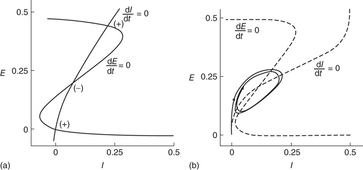
Figure 22.7 (a) phase plane and null clines of the mean-field Wilson–Cowan equations. The intersections of the two null clines are equilibrium or fixed points of the equations. Those labeled are stable, those labeled are unstable. Parameters: . The stable fixed points are nodes. (b) Equilibrium which is periodic in time. Parameters: . In this case, the equilibrium is a limit cycle. (Redrawn from [3].)

There is also another phase plane portrait in which the equilibrium is as a damped oscillation, that is, a stable focus. In fact, by varying the synaptic weights and or and , we can move from one portrait to another. It turns out that there is a substantial literature dealing with the way in which such changes occur. The mathematical technique for analyzing these transformations is called bifurcation theory, and it was first applied to neural problems 52 years ago [15], but first used systematically by Ermentrout and Cowan [16–18] in a series of papers on the dynamics of the mean-field Wilson–Cowan equations.

More detailed studies of neural bifurcation in the Wilson–Cowan equations were subsequently carried out by Borisyuk and Kirillov [20], and Hoppensteadt and Izhikevich [19]. The left panel of Figure 22.8 shows a representation of the detailed structure of such bifurcations. It will be seen that the saddle–node and Adronov–Hopf bifurcations lie quite close to the Bogdanov–Takens (BT) bifurcation. This implies that all the bifurcations of the Wilson–Cowan equations we have described are fairly close to the BT bifurcation, in the (a, b)-plane.

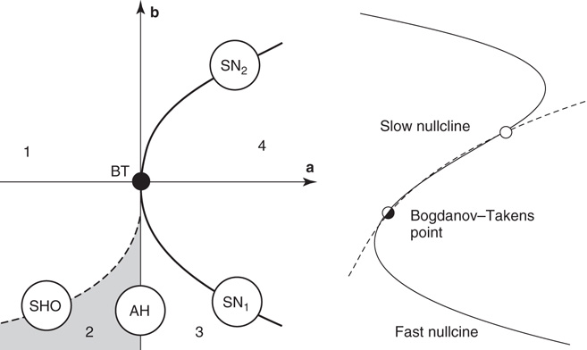
Figure 22.8 (a) Bifurcations of the Wilson–Cowan equations organized around the Bogdanov–Takens (BT) bifurcation. SN1 and SN2 are saddle–node bifurcations. AH is an Andronov–Hopf bifurcation, and SHO is a saddle homoclinic–orbit bifurcation. Note that a and b are control parameters, either synaptic weights or their products, as described in the caption to Figure 22.7. (b) Nullcline structure at a Bogdaov–Takens bifurcation. At the Bodanov–Takens point, a stable node (open circle) coalesces with an unstable point. (Redrawn from [19].)

The BT bifurcation depends on two control parameters, and is therefore said to be of co-dimension 2. It has the property that an equilibrium point can simultaneously become a marginally stable saddle–node bifurcation point and an Andronov–Hopf bifurcation point. Thus at the critical point, the eigenvalues of its associated stability matrix have zero real parts.

In addition, the right panel of Figure 22.8 shows the way in which the fast -nullcline and the slow -nullcline intersect. The point of first contact of the two nullclines is the BT point. It will be seen that there is region of the phase plane above this point where the two nullclines remain close together. This is a defining characteristic of such a bifurcation. Interestingly, it is closely connected with the balance between excitatory and inhibitory currents, as was noted in Benayoun et al.'s study of avalanches in stochastic Wilson–Cowan equations [13]. This is another demonstration that avalanches with a power law distribution are generated in stochastic neural networks close to critical points, and therefore lie in the fluctuation-dependent region of a phase transition. In the case of stochastic neural networks, our results suggest that the phase transition belongs to the directed percolation universality class.

22.4 An E–I Neural Network Exhibiting Self-Organized Near-Criticality

We now consider the neural patch or module shown in Figure 22.9. Again, we note that this module is spatially homogeneous. We model the neocortical sheet as a two-dimensional network or array of such circuits. In such an array, note that the neighboring excitation provides the recurrent excitatory connection. This requires , so that the recurrent excitatory connection shown in Figure 22.9 (not labeled) has strength . The recurrent inhibitory connection (also unlabeled) takes the value . The basic equations for the array thus take the form of Eqs. (22.13) and (22.14), except that the activities and are now functions of position, as are the excitatory and inhibitory currents and which are given by the expressions

where runs over all nearest neighbor patches.

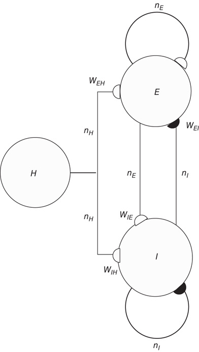
Figure 22.9 A recurrent network module driven by the input , acting through the synaptic weight and .

Note also that the density of inter-patch and connections is very small relative to that of connections, so we have neglected them in calculating the excitatory and inhibitory currents and .

22.4.1 Modifiable Synapses

We now introduce generalized Vogels equations for the four internal synaptic weights in each patch, , and . The excitatory synapses and are assumed to be anti-Hebbian, and the inhibitory synapses and Hebbian. Mean-field equations for these weights take the following form:

22.15

where and run over the set , and the coefficients and give the transitions rates for the Markov processes governing the four weights. These take the form

22.16

for the excitatory anti-Hebbian weights, and

22.17

for the inhibitory Hebbian weights. Note that for such weights .

In the continuum limit, these equations take the form

22.18

for excitatory weights, and

22.19

for inhibitory weights.

22.4.2 A Simulation of the Combined Mean-Field equations

The complete set of mean-field equations for an patch with modifiable weights comprises the Wilson–Cowan equations 22.14 together with the generalized Vogels Eqs. 22.18 and 22.19, supplemented by the modified current equations given above, for the full two-dimensional array. Such a system of equations can be simulated, and the results are shown in Figure 22.10.

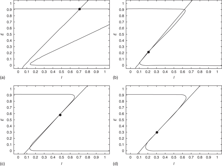
Figure 22.10 phase plane and null clines of the mean-field Wilson–Cowan equations. The intersections of the two nullclines in each panel are equilibrium or fixed points of the equations. (a) Initial state at s with weights . There is a stable fixed point at . (b) State at s with weights . There is now a saddle point at . (c) State at s, with weights , and a saddle point at . (d) Final state at s, with weights , with a stable fixed point at . The remaining fixed parameters are .

It will be seen that a single patch self-organizes from one stable fixed point defined by the initial conditions to another stable fixed point at which , as expected. We note that, in case the initial conditions are constrained so that and , and all the fixed parameters of the population equal those of the population, then the final state is also similarly constrained. We refer to this as a symmetry of the system. Given such a symmetry and the target condition , it follows that , so that

Thus the combined system is homeostatic. It self-organizes so that the strengths of all the synaptic weights stay within a certain range. The homeostatic properties of anti-Hebbian synapses were previously noted by Rumsey and Abbott [21].

22.4.3 Balanced Amplification in Patches

This inequality has a number of important consequences [13, 22]. In particular, it leads to a particular change of variables in the relevant Wilson–Cowan equations. Consider such equations for a single patch, given the symmetry described above:

22.20

where , and and are interpreted as the fractions of activated and neurons in a patch.

Now introduce the change of variables

22.21

so that Eq. 22.20 transforms into

22.22

Such a transformation was first introduced into neural dynamics by Murphy and Miller [22], and followed by Benayoun et al. [13]. But it was actually introduced much earlier by Janssen [23] in a study of the statistical mechanics of stochastic Lotka–Volterra population equations on lattices, which are known to be closely related to stochastic Wilson–Cowan equations [24]. Interestingly, Janssen concluded that systems of interacting predator and prey populations satisfying the Lotka–Volterra equations exhibited a nonequilibium phase transition in the universality class of directed percolation, just as we later demonstrated in stochastic Wilson–Cowan equations [25]. Janssen used the transformed equations to show that, in the neighborhood of such a phase transition, only the variable survives.

To show this, we note that the transformed equations are decoupled with the unique stable solution . In turn, this implies that at such a fixed point in the original variables. This is precisely the stable fixed point reached in the simulations shown in Figure 22.11. In addition, it also follows that the fixed-point current in the new variables is

So at the stable fixed point , , and in fact, near such a fixed point, is only weakly sensitive to changes in , and is unchanged by varying while keeping constant. For all these reasons, Murphy and Miller described the decoupled equations as an effective feed-forward system exhibiting abalance between excitatory and inhibitory currents, and a balanced amplification of any stimulus .

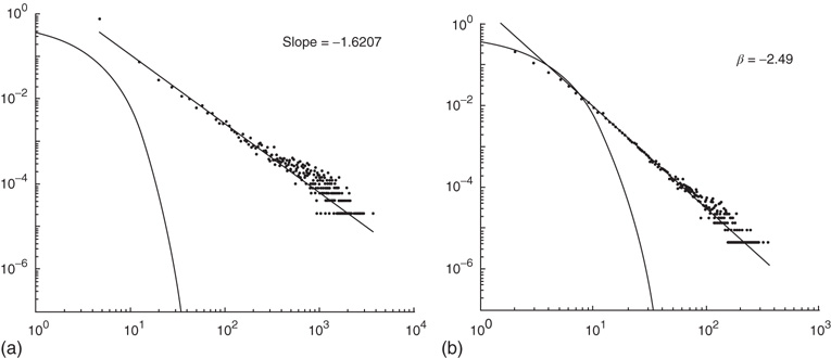
Figure 22.11 (a) Avalanche distribution in the all-to-all case. The distribution is approximately a power law with a slope (blue line). For comparison, a Poisson distribution is plotted. (b) Avalanche distribution in the sparsely connected case. The distribution is approximately another power law with a slope of . Note that both distribution show bulges at large avalanche sizes.

22.4.4 Analysis and Simulation of the Combined Markov Processes

It remains to analyze and simulate the statistical dynamics of the coupled Markov processes introduced earlier to represent the effects of fluctuations in both neural activity and in synaptic plasticity. But the various synaptic weights have strengths that depend on neural activity. So the characteristics of such activity determine those of the weights. But we have shown for patches that the combined mean-field dynamics reaches a stable equilibrium in the form of a node, and that at this node there is a balance reached between excitation and inhibition. We can obtain more information about the properties of this node by considering the effects of small deviations or fluctuations in the activity.

To do this, we now start from the fact the fixed point is a stable node. This means that we can expand the master equation directly via the van Kampen system-size expansion [4]. This expansion was first used in the neural context by Ohira and Cowan [26] and later by Bressloff [27] and Benayoun et al. [13]. Thus we do not need to use the methods of statistical field theory for this part of the analysis. The details of the system-size expansion are straightforward. Since the fixed point is stable, we can assume that small fluctuations about such a fixed point are Gaussian. Thus the fractions of activated excitatory and inhibitory neurons at time can be written as

22.23

where are, respectively, the numbers of excitatory and inhibitory neurons, are, as before, the mean fractions of activated excitatory and inhibitory neurons, and are stochastic perturbations. The mean fractions satisfy Eq. 22.20, and the mean current is as before. The stochastic variables satisfy the (linear) Langevin equation

22.24

or in the transformed variables

22.25

where the eigenvalues are and , and . The Jacobian matrix

is upper triangular and has eigenvalues and . It follows that, when is small and positive, then so are the eigenvalue magnitudes and . So the eigenvalues are small and negative, and the fixed point is weakly stable. Evidently, lies close to the matrix

But the matrix is the signature of the normal form of the BT bifurcation [19]. Thus the weakly stable node lies close to a BT bifurcation, as we have suggested. The stochastic interpretation of this is that the weakly stable node lies close to the critical point of a phase transition in the universality class of directed percolation. (Note that we cannot perform a system-size expansion of the master equation in case the fixed point is only marginally stable, as it is at a critical point. This situation required the renormalization group treatment [9].)

To simulate the combined Markov processes described by such a stochastic system, [13] used the Gillespie algorithm to simulate the stochastic behavior of two architectures: (i) an all-to-all connected patch comprising excitatory and inhibitory neurons (these are the proportions of such neurons in the neocortex). The results are shown in Figure 22.11a; (ii) a sparsely connected patch in which random sparse positive matrices with large eigenvalues, and with small eigenvalues are generated so that the overall weight matrix

is random. (The condition that the eigenvalues of are much greater than those of is equivalent to the condition in the all-to-all case.) The result is shown in the right panel of Figure 22.11. (iii) We do not yet have a finished simulation of the two-dimensional case, but we conjecture that the results will be similar in that the avalanche distribution will be approximately a power law, but with a slope of . (See also the recent paper by Magnasco et al. [28].)

22.5 Discussion

We have demonstrated the following properties of stochastic Wilson–Cowan equations: (i) A simple two-dimensional array comprising patches of excitatory neurons driven by a weak external stimulus acting through a modifiable anti-Hebbian synapse self-organizes into an oscillation between two stable states, an UP state of high neural activity and a DOWN state of low activity, each of which loses its stability at the critical point of a nonequilibrium phase transition in the universality class of directed percolation. Such noisy oscillations generate bursts or avalanches of neural activity whose avalanche distributions are consistent with such a phase transition. (ii) We then analyzed the properties of a array comprising patches of both excitatory and inhibitory neurons, with excitatory anti-Hebbian and inhibitory Hebbian synapses. We found that the spontaneous-fluctuation-driven activity of a single patch self-organizes to a weakly stable fixed point. However, such a fixed point lies close to a marginally stable fixed point. Thus we conclude that the effect of Hebbian inhibition is to stabilize the dynamics of the patch, but that the statistical dynamics of the patch remains within the fluctuation drive regime surrounding the critical point of a nonequilibrium phasetransition, which again is in the universality class of directed percolation. (We are preparing a manuscript contained a detailed analysis of this situation using renormalization group techniques, along the lines of Janssen's analysis of stochastic Lotka–Volterra equations.) (iii) We have also shown that the mean-field dynamics of the case can be analyzed around the BT bifurcation, and that the generalized Vogels equations for Hebbian and anti-Hebbian plasticity drive the patch dynamics to a weakly stable node near such a bifurcation, and in doing so reduce the dynamics to the dynamics of a single patch.

In summary, we conclude that an array of -patches will self-organize around critical points of the directed percolation phase transition and, when driven by a weak stimulus, will oscillate between an UP state and a DOWN state each of which generates avalanches consistent with directed percolation. The array therefore exhibits SOC and replicates the behavior of the original sandpile model of [1]. We can also conclude that an array of patches will also self-organize to a weakly stable node located near the critical point of a directed percolation phase transition so that fluctuations about the weakly stable node will also follow a power slope with a slope characteristic of directed percolation. We refer to this as SONC. We note that there is some experimental evidence to support this conclusion [29, 30].

Acknowledgements

Some of the work reported in this paper was initially developed (in part) with Hugh R. Wilson, and thereafter with G.B. Ermentrout, then with Toru Ohira, and later with Michael A. Buice. The current work was supported (in part) by a grant to Wim van Drongelen from the Dr. Ralph & Marian Falk Medical Trust.

References

1. 1. Bak, P., Tang, C., and Wiesenfeld, K. (1988) Self-organized criticality. Phys. Rev. A, 38, 364–374.
2. 2. Gil, L. and Sornette, D. (1996) Landau-ginzburg theory of self-organized criticality. Phys. Rev. Lett., 76 (21), 3991–3994.
3. 3. Wilson, H. and Cowan, J. (1972) Excitatory and inhibitory interactions in localized populations of model neurons. Biol. Cybern., 12, 1–24.
4. 4. Van Kampen, N. (1981) Stochastic Processes in Physics and Chemistry, North Holland.
5. 5. Wilson, K. (1971) Renormalization group and critical phenomena. I. renormalization group and the kadanoff scaling picture. Phys. Rev. B, 4 (9), 3174–3183.
6. 6. Cowan, J., Neuman, J., Kiewiet, B., and van Drongelen, W. (2013) Self-organized criticality in a network of interacting neurons. J. Stat. Mech., P04030.
7. 7. Hinrichsen, H. (2000) Non-equilibrium critical phenomena and phase transitions into absorbing states. Adv. Phys., 49 (7), 815–958.
8. 8. Korolev, K. and Nelson, D. (2011) Competition and Cooperation in one-ddimensional stepping-stone models. Phys. Rev. Lett., 107 (8), 088–103.
9. 9. Buice, M. and Cowan, J. (2007) Field theoretic approach to fluctuation effects for neural networks. Phys. Rev. E, 75, 051–919.
10. 10. Vogels, T., Sprekeler, H., Zenke, F., Clopath, C., and Gerstner, W. (2011) Inhibitory plasticity balances excitation and inhibition in sensory pathways and memory networks. Science, 334 (6062), 664–666.
11. 11. Han, V.Z., Grant, K., and Bell, C. (2000) Reversible associative depression and nonassociative potentiation at a parallel fiber synapse. Neuron, 24, 611–622.
12. 12. Gillespie, D. (2000) The chemical Langevin equation. J. Chem. Phys., 113 (1), 297–306.
13. 13. Benayoun, M., Cowan, J., van Drongelen, W., and Wallace, E. (2010) Avalanches in a stochastic model of spiking neurons. PLoS Comput. Biol., 6 (7), e1000846.
14. 14. Wilson, H. and Cowan, J. (1973) A mathematical theory of the functional dynamics of cortical and thalamic nervous tissue. Kybernetik, 13, 55–80.
15. 15. Fitzhugh, R. (1961) Impulses and physiological states in theoretical models of nerve membrane. Biophys. J., 1, 445–466.
16. 16. Ermentrout, G. and Cowan, J. (1979b) Temporal oscillations in neuronal nets. J. Math. Biol., 7, 265–280.
17. 17. Ermentrout, G.B. and Cowan, J.D. (1979a) A mathematical theory of visual hallucinations. Biol. Cybern., 34, 137.
18. 18. Ermentrout, G.B. and Cowan, J.D. (1980) Large scale spatially organized activity in neural nets. SIAM J. Appl. Math., 38 (1), 1–21.
19. 19. Hoppensteadt, F. and Izhikevich, E. (1997) Weakly Connected Nrural Nnetworks, MIT Press, Cambridge, MA.
20. 20. Borisyuk, R. and Kirillov, A. (1992) Bifurcation analysis of a neural network model. Biol. Cybern., 66 (4), 319–325.
21. 21. Rumsey, C. and Abbott, L. (2004) Synaptic equalization by anti-STDP. Neurocomputing, 58-60, 359–364.
22. 22. Murphy, B. and Miller, K. (2009) Balanced amplification: a new mechanism of selective amplification of neural activity patterns. Neuron, 61 (4), 635–648.
23. 23. Janssen, H. (2001) Directed percolation with codors and flabors. J. Stat. Phys., 103 (5-6), 801–839.
24. 24. Cowan, J.D. (2013) A personal account of the development of the field theory of large-scale brain activity from 1945 onward, in Neural Fidld Theory (eds S., Coombes, P. BiemGraben, R. Potthast, and J. Wright), Springer, New York.
25. 25. Buice, M. and Cowan, J. (2009) Statistical mechanics of the neocortex. Prog. Biophys. Theor. Biol., 99 (2,3), 53–86.
26. 26. Ohira, T. and Cowan, J.D. (1997) Stochastic neurodynamics and the system size expansion, in Proceedings of the First International Conference on the Mathematics of Neural Networks (eds S. Ellacort and I. Anderson), Academic Press, pp. 290–294.
27. 27. Bressloff, P. (2009) Stochastic neural field theory and the system-size expansion. SIAM J. Appl. Math., 70 (5), 1488–1521.
28. 28. Magnasco, M., Piro, O., and Cecchi, G. (2009) Self-tuned critical anti-hebbian networks. Phys. Rev. Lett., 102, 258–102.
29. 29. Tagliazucchi, E., Balenzuela, P., Fraiman, D., and Chialvo, D. (2012) Criticality in large-scale brain fMRI dynamics unveiled by a novel point process analysis. Front. Physiol., 3, 1–12.
30. 30. Haimovici, A., Tagliazucchi, E., Balenzuela, P., and Chialvo, D. (2013) Brain organization into reating state nnetworks emerges at crituality on a Model of the human connectiome. Phys. Rev. Lett., 110, 178–101.