 BEFORE CONTINUING, WRITE DOWN A PERCENTILE THAT REPRESENTS THE PROBABILITY YOU WILL STEAL THE DIAMOND.
Probability is one of the more difficult concepts for humans to understand and deal with effectively. Morton Hunt explained why in The Universe Within. He wrote:
Most of the concepts and patterns that are difficult for the average person to grasp and use are “nonintuitive”—that is, they cannot be derived, or are not easily derived, from everyday experience, and therefore are not part of the normal mind’s repertoire. Probability is one such [concept]; most people can intuitively see the answer to only the simplest problems involving probability.
Jeremy Campbell in The Improbable Machine made a similar observation:
People do not seem to learn, easily or at all, the rules of probability … just by having repeated experiences of them…. [One explanation for this] seems to be that the rules of… probability fly in the face of common sense. And “common sense” in many cases turns out to mean the way in which human memory is organized and how it processes information.
Thinking in Time by Harvard professors Neustadt and May was equally discouraging:
Judging by our students, millions of Americans are either unfamiliar with numerical notations of probability or are uncomfortable at the idea of stating a subjective judgment [in terms of probability].
The reason we humans have difficulty with probability calculations and estimates is that our brains (our minds) are not equipped with a “probability module.” We can intuitively and fairly accurately estimate the height of most objects, like a tree or ladder. We can estimate distances like the dimensions of a room. These estimates rely on visual perceptions, with which we are innately comfortable and confident. But when it comes to the nonvisual, intangible process of estimating probability, we are notoriously unreliable. What it comes down to is that the human mind was not designed to think in terms of mathematical probability. For that reason we must be wary of our intuitive judgments involving probability because they can drastically mislead us.
For example, we humans tend to believe that, because an event took place, it was highly likely to take place. If the weather bureau forecasts only a 5 percent chance of rain, and we go on a picnic and get drenched in a downpour, we instantly conclude that the weather bureau goofed. Obviously the probability of rain was higher than 5 percent. More like 100 percent. Look at us! We’re soaked! But what does a 5 percent chance of rain really mean? It means that weather history gathered over decades shows that 5 percent of the time, when meteorological conditions like the ones we are experiencing prevail, it rains. Expressed another way, if these exact weather conditions are repeated many, many times, 5 percent of those many, many times it will rain. It means the downpour that soaked us was one of the 5 percent. It doesn’t mean the forecast was wrong; it means our intuition is wrong.
Understanding and dealing with probability are crucial because probability permeates analysis both explicitly and implicitly. It lies hidden in the information we analyze and is a crutch for our analytic judgments. Unless we are sensitive to probability’s influence and accurately define its meaning and significance, it can, like a computer virus devouring computerized data, devastate our analytic findings and make a mockery of our recommendations and decisions.
As I mentioned earlier, the most difficult analytic problems are of the random and indeterminate type, where, because facts are scarce, our analytic product depends heavily on subjective judgments. For that reason, there can be no certainty when dealing with random or indeterminate problems. No certainty at all! The moment our analysis moves from facts to judgment, we leave certainty behind and enter the arena of estimates. “Estimating is what we do when we run out of data. The language of estimating is probability, and the laws of probability are the grammar of that language.” So said the late Sherman Kent, a U.S. intelligence officer widely regarded as the “father” of the National Intelligence Estimate.
Probability is difficult to deal with because the laws of probability, as Hunt observed, are often counterintuitive and the judgments resulting from the application of those laws are, more often than not, imprecise and ambiguous when expressed verbally.
With that ambiguity in mind, and as a prelude to further discussion of probability, do the following exercise:
A fabulous diamond is kept in a safe behind five doors, each secured by a combination lock. You are a thief seeking to steal the diamond. All five doors have exactly the same kind of lock made by the same company but with different combinations. In your career as a thief, you have encountered this lock ten times. Only once—the last of those ten times—have you failed to open the lock. Disregarding all factors except the combination lock, what is the probability, expressed as a percentile (20%, 50%, 80%, etc.), that you will get through all five doors and steal the diamond? Write your percentile on a sheet of paper.
BEFORE CONTINUING, WRITE DOWN A PERCENTILE THAT REPRESENTS THE PROBABILITY YOU WILL STEAL THE DIAMOND.
Next to your percentile, write an adjective or adverb-adjective that you think best characterizes the percentile, such as unlikely, possible, very likely, almost certain.
BEFORE CONTINUING, WRITE NEXT TO THE PERCENTILE AN ADJECTIVE OR ADVERB-ADJECTIVE THAT CHARACTERIZES THE PERCENTILE. (KEEP THE SHEET OF PAPER. WE’LL REFER TO IT LATER.)
People commonly make inordinately casual use of probability expressions, such as most likely, in all likelihood, may, slim chance, and certainly, under the mistaken assumption that these expressions mean the same thing to everyone.
“What are our chances of being on time for our appointment if we stop for dinner?” asks a wife of her husband.
“Fair,” he replies.
“Okay,” she says, “then let’s stop here.”
After dining, they arrive at their appointment a half hour late. She’s upset and complains to her husband, “I thought you said we’d be on time!”
He’s shocked. “I never said anything of the kind.”
“You said our chances were ‘fair.’ “
“Yeah, like we wouldn’t be on time!”
People unfortunately have drastically different perceptions of what nonnumeric (adjectival) expressions of probability mean. Ask people how they interpret likely as a numerical percentage and you’ll get answers ranging from 55 to 85 percent. What’s a slight chance of rain? To the public at large, anywhere from 1 to 15 percent. If you’re skeptical of these ranges, do your own survey. Ask your family or friends what various adjectival probability terms mean to them. You’ll find their responses enlightening and entertaining.
Whether we are analyzing a problem alone or collaborating with others, we should make it a rule to highlight all probability expressions and translate them into percentiles. I’ve italicized certain words in the following excerpt of an article in Firehouse magazine to show you what I mean:
The U.S. Fire Administration’s Juvenile Firesetter Programs show that the greater percentage of fires are set by young children in the five to nine age group. In addition, these programs indicate that five- and six-year-olds may not be capable of understanding the concept that a single match can destroy a house. Therefore, not only do young children represent the highest risk group with respect to their involvement in firestarting, but they are also the most likely victims of fire injury and death…. Unlike elementary school children, who may be involved in only one or two unsupervised firestarts, psychiatric patients are more likely to be involved in several incidents of firesetting behavior. In addition, the fires set by children with psychiatric diagnoses are more likely to cause serious damage requiring firefighter suppression.
This is a typical example of casual use of probability expressions. If they weren’t highlighted, they would hardly be noticed. Yet because they have significant impact on the meaning of the text, it is fair to question what precise probability the authors meant to convey in each case.
[S]ix-year-olds may not [understand] that a single match can destroy a house.
What probability do the authors assign to “may”? Fifty percent? Ten percent? One percent? It makes a huge difference. If there’s a 50 percent chance that America’s six-year-olds do not appreciate the dangerous firepower of a single match, the nation’s homes are in serious jeopardy. If, on the other hand, there’s only a 1 percent chance, the danger is drastically reduced.
[Y]oung children … are the most likely victims of fire.
What does “most likely” mean? Sixty percent? Eighty percent? Ninety-nine percent?
I repeat my advice. When we are analyzing a problem or drafting a report, we should convert all probability expressions into percentiles… but only in the analytic phase. Never use percentiles in final written products unless—and such instances are extremely rare—the numbers are based on definitive evidence and precise calculations. The biggest challenge in dealing with probability is conveying through language what a probability represents without using a percentile. But that’s a subject for a book on writing, not a book on structuring analysis. (One solution, favored by some writers and strongly opposed by some others, is to identify up front for the reader what the various probability expressions used in a written product represent in percentiles, e.g., “probable” = 85%, “unlikely” = 20%, etc.)
How do we determine probability? There are basically two ways: computation and frequency-and-experience. When we have all the facts, that is, when we have all of the data, as in a deterministic problem, we calculate probability by arithmetic computation. When we don’t have all the facts, we estimate probability based on frequency and experience. Frequency is how often an event has occurred in the past; experience is what happened during each event. A simple example: If I drop ten lightbulbs, one at a time, on the floor and each one breaks, what’s the probability that, if I drop an eleventh bulb, it too will break? Very high! Almost 100 percent. How did I reach that conclusion? Frequency—I repeated the event ten times. Experience— the bulbs broke every time.
Obviously, the more we know about the circumstances of an event whose probability we are estimating, the more accurate our estimate will be. But what if we know little or nothing about the circumstances? What if someone asked you to estimate which of three political parties will win a coming election in Tanganyika, Africa? Unless by chance you are a student of African affairs, you won’t have the slightest idea. A French nobleman, Marquis Pierre-Simon de Laplace (1749-1827), gave us sound advice about how to deal with such a situation. According to Laplace, if we’re trying to determine which of two or more outcomes will occur, but we don’t have reliable evidence to judge which is more likely, we should assume the probability is equal for all outcomes. Let me repeat: if we lack evidence to support a judgment as to which of two or more outcomes is most likely, we should assume that all are equally likely.
Fortunately, we rarely have occasion to resort to Laplace. In almost every problem we face, we recognize similarities with past events of which we have some knowledge, and we use that knowledge as the basis for making probability judgments (estimating probabilities). However, our probability estimates are as vulnerable as any other workings of the human mind to those troublesome mental traits I’ve been talking about. “Similarities with past events” are often among those nonexistent patterns our minds are prone to perceive. And as we are prone to value evidence that supports a favored outcome, so are we prone to believe that a favored outcome is more likely (has a greater probability of occurring) than one unfavored. And we are likely to hold fast to this belief in the face of contrary evidence. Yes, indeed, our minds can as easily mislead our probability estimates as they can any other analytic judgment.
A memorably poignant example of this tendency to inflate the probability of a desired outcome was revealed in a statement by a British Royal Navy commando who took part in the Normandy invasion in World War II. “I don’t think any of us realized the danger we were in. Nobody ever went to Normandy to die; they went to fight and win a war. I don’t think any man that died thought that it was him that was going to be killed.” Inflating or deflating probabilities to conform to our desires is the curse of wishful thinking: it won’t happen to me because I don’t want it to happen. As Francis Bacon said, we prefer to believe what we prefer to be true.
Given the absolutely crucial role of probability in the analysis of problems, we must take great care in the determination of probability assessments.
The two most common types of events whose probability we try to determine when analyzing problems are mutually exclusive and conditionally dependent.
Mutually exclusive events preclude one another. For example, the tossing of a coin involves mutually exclusive events, or mutually exclusive outcomes. Because a coin has two sides, one outcome (heads or tails) precludes the other. The outcomes are thus mutually exclusive. Rolling a standard die also involves mutually exclusive events. A standard die has six faces, only one of which can “come up.” One outcome thus precludes the others. Election outcomes are mutually exclusive, as is almost every decision we humans make every day. If we decide this, we exclude that.
Conditionally dependent events are those in which the occurrence of one event depends upon the occurrence of another. The events thus occur in sequence. Starting the engine of an automobile is a good example. We insert the key into the ignition switch, we turn the key, the starter rotates the engine, and the engine ignites. The engine won’t ignite if it isn’t rotated; the starter won’t rotate the engine unless we turn the ignition key; we can’t turn the key unless we insert it into the ignition switch. The first event—inserting the ignition key—conditions the second, meaning the second event occurs on condition that the first occurs. The second event conditions the third, and so on.
How do we calculate mutually exclusive probability? A useful vehicle for explaining this calculation is a jar containing 90 jelly beans: 45 red ones, 36 yellow, and 9 green. We’re going to reach into the jar and pick out one bean. We can visualize this more clearly with a scenario tree (Figure 13-1) in which we have three possible, mutually exclusive decisions or outcomes: red, yellow, and green.
FIGURE 13-1
Assuming the beans are distributed randomly, what is the probability, if I reach into the jar and blindly take out a single jelly bean, that it will be red? What probability yellow? What probability green?
One easy way to compute mutually exclusive probabilities is to think of them as percentages. For example, the probability of picking one red bean out of 90 in one try is equal to the percentage of the 90 that are red. Does that make sense? Maybe it’s clearer if I rephrase the sentence. If 30 percent of the beans in the jar are red, then I have a 30 percent chance of picking a red bean on one try.
How, then, do we compute the percentage of red beans in the jar? I like to use the traditional IS-over-OF method: IS divided by OF. I learned it in grade school and have never found a better way to structure the arithmetic formula. (Yes, IS-over-OF is a structuring technique.) To do the calculation, we ask ourselves, “What percent is this number of that one?” We then divide the IS number by the OF number. For instance, what percent is 3 of 6? Or what percent of 6 is 3? IS (3) over OF (6): 3 divided by 6 equals .5 (50 percent).
One advantage in using the IS-over-OF formulation is that sometimes the context of a problem makes it difficult to determine which number is to be divided by which. I was taught, when encountering this dilemma, to transform the language of the problem into an IS-over-OF format. To whit, a bushel contains 40 apples, 10 of which are rotten. What percentage are rotten? Some people might be confused as to which number is the divisor and which the dividend. To find out, one simply rewords the question as follows: What percent is 10 of 40? IS-over-OF; 10 over 40 = .25 (25 percent). I love it! (God bless my grade school teachers.)
Let’s apply the IS-over-OF formula to the question of what percentage of the jelly beans in the jar are red, what percentage yellow, and what percentage green. Compute the answers and write them on a sheet of paper.
BEFORE CONTINUING, COMPUTE THE PERCENTAGE OF RED, YELLOW, AND GREEN BEANS.
Here are the answers:
Red—What percent is 45 of 90? IS (45) over OF (90) = .5 or 50 percent.
Yellow—What percent is 36 of 90? IS (36) over OF (90) = .4 or 40 percent.
Green—What percent is 9 of 90? ÍS (9) over OF (90) = .1 or 10 percent.
Now we convert the percentages to probabilities and enter the numbers in the tree (Figure 13-2).
Because the tree contains probabilities, I prefer to call it a “Probability Tree.”
A probability tree has all the attributes of a scenario tree plus one: It enables us to analyze the entire tree and any of its elements from the perspective of probability. It further enables us to estimate which scenario is most likely and which is least likely, and which decisions and events within the alternative scenarios are most likely and least likely. Whereas a scenario tree shows only what can and cannot happen, a probability tree shows what is likely and unlikely to happen. Adding probability as a dimension to our analysis therefore instills reality in our findings.

FIGURE 13-2 Probability Tree
A probability tree, moreover, highlights and allows us to focus our attention on, collect evidence on, challenge the assumptions on, those decisions and events that determine the viability of scenarios that are important to us. We can enhance our ability to identify these determinants by arbitrarily varying the probabilities we assign them—doing what is called sensitivity analysis. A probability tree can therefore show us on which decision or event we should concentrate our effort if we wish to increase the likelihood of a particular scenario. Imagine the immense value and power of knowing where to concentrate one’s effort to bring about an outcome we favor.
There are three inviolable rules for constructing probability trees:
As with any scenario tree, the events depicted must be mutually exclusive, meaning each event is distinct from the others.
Likewise, the events must be collectively exhaustive, meaning they must include all possible events in the scenario being analyzed.
The probabilities of the branches at each node (each branching of the tree) must equal 1.0.
A point to remember for those unaccustomed to dealing with, and calculating, numerical probabilities is that an event cannot occur more times than its possibility of occurring. Therefore, probability can never be greater than 100 percent, or 1.0.
Let’s raise the complexity of the jelly bean problem a notch.
What is the probability of picking a red or a green jelly bean from the jar in one try?
Again, the way to solve this problem is to think in terms of percentages: what percent of the beans in the jar are red or green? There are 45 red and 9 green, which equals 54. What percent of 90 is 54? IS (54) over OF (90) = .6. So we have a .6 probability of picking red or green on one try. What we did, in effect, was to add the probability of picking a red (.5) and the probability of picking a green (.1).
What is the probability of picking a red or a yellow? What is the probability of a yellow or a green? Write your answers on a sheet of paper.
BEFORE CONTINUING, COMPUTE THE PROBABILITY OF PICKING RED OR YELLOW, YELLOW OR GREEN BEANS
The probability of picking red or yellow is .5 + .4 = .9
The probability of picking yellow or green is .4 + . 1 = .5
The point here is that we express OR in probability calculations as a plus sign; that is, we add the OR probabilities. This is one of those probability concepts that most analysts don’t understand until it is called to their attention, meaning it isn’t intuitively obvious. Even when the concept is pointed out, it doesn’t sink in for many people. As Campbell wrote, people don’t seem to remember the rules of probability simply by practicing them. That’s why most of us have to reason them out every time.
Let’s practice drawing a probability tree and calculating an OR probability.
Fifty hens live in a henhouse: 10 are red, 5 are black, 15 are brown, and 20 are white. If a fox steals into the henhouse and randomly kills a hen, what is the probability the hen will be red or brown? On a separate sheet of paper, draw a probability tree showing each color hen’s probability of being killed and then determine the answer to the problem.
BEFORE CONTINUING, CONSTRUCT A PROBABILITY TREE AND COMPUTE THE PROBABILITY THE HEN KILLED WILL BE RED OR BROWN.
Figure 13-3 shows the probability tree.
The probability of killing a red hen is .2 and a brown hen is .3, so the probability of killing either a red or a brown is .2 + .3 = .5.
How do we calculate conditionally dependent probability? By multiplying the two probabilities that are linked conditionally. Let me explain why.
What is the probability of tossing two heads in a row with a coin?
The probability tree in Figure 13-4 illustrates the possible sequences of events. The probability of getting heads on the first toss is .5. If we get tails, the sequence ends; it’s over, and we’re stuck on that limb of the tree. We toss the coin a second time only on condition that we get heads on the first toss. Thus, the second toss is conditionally dependent upon the first. If we get heads on the first toss, what is the probability of getting heads on the second toss? Still .5, so we have a 50 percent chance of a 50 percent chance (.5 times .5) of tossing two heads in a row, which equals a probability of .25.

FIGURE 13-3
FIGURE 13-4
Let’s review calculating conditionally dependent probability with the jelly beans. What is the probability that we will first pick a single red bean (and return it to the jar) and then pick a green bean? Figure 13-5 portrays this sequence. The probability of picking a single red bean is .5; the probability of a single green bean is .1. So the probability of picking a red and then a green bean is .5 times .1, which equals .05.
Let’s go back to the “Safecracker” problem. There were five doors, each secured by a combination lock. You, the thief, had picked this kind of lock on nine of ten previous occasions. You failed only once, the tenth try. What is the probability you will unlock all five doors?
This is a problem of conditionally dependent probabilities, because opening the second door is dependent upon opening the first, opening the third is dependent upon opening the second, and so on.
What is the probability (let’s call it PI) you will get through the first door? We compute it based on your previous success rate: 9 out of 10. What percent is 9 of 10? 90. So PI is .9.

FIGURE 13-5
What is the probability of opening the first and second doors? Opening the second door is contingent upon opening the first. We therefore multiply the probability of opening the first door (.9) times the probability of opening the second. What is the probability of opening the second door? .9? Sorry, wrong number. That was the probability of the first door based on nine out of ten successes. But if we opened the first door we scored another success, so now our batting average is 10 divided by 11, which is .91. The answer to the probability of opening the first two doors is .9 times .91, which is .82. Are you following this? If not, read the foregoing again.
Calculate the probability of opening the fifth door (and, of course, stealing the diamond). Write your calculations and final answer on a sheet of paper.
BEFORE CONTINUING, CALCULATE THE PROBABILITY OF OPENING THE FIFTH DOOR.
The following list provides the answers.
P1 is 9 divided by 10 = .9.
P2 is .9 times 10 divided by 11 = .82.
P3 is .82 times 11 divided by 12 = .75.
P4 is .75 times 12 divided by 13 = .69.
P5 is .69 times 13 divided by 14 = .64.
Now compare .64 with the percentile you earlier selected to represent the probability of your stealing the diamond. How close were you? Most people intuitively believe the probability of stealing the diamond is quite high. If you earlier greatly miscalculated the probabilities in the Safecracker I problem, don’t be upset. Most people miscalculate them because, as I said at the opening of this chapter, probability is one of the more difficult concepts for humans to understand and deal with effectively. It is unquestionably not instinctive. For that reason, we must thoroughly understand the differences in the concepts of mutually exclusive and conditionally dependent probabilities, and we must practice calculating these probabilities every chance we get. Only by doing so will they become second nature to us.
The distinction between calculating mutually exclusive and conditionally dependent probabilities is clearly apparent in how we diagram these two calculations in a probability tree.
In summary, to determine the combined probability that two or more events will occur as a result of a single decision or event (the “or” situation), we add their individual probabilities. To determine the probability that two or more events will occur in succession (the “and” situation), we multiply their individual probabilities.
In dealing with probability questions, we must carefully scrutinize how a probability statement or question is framed, that is, whether the question relates to the probability of a single (mutually exclusive) event or a series of connected (conditionally dependent) events. Wording of the probability question is critical and underlines the importance of restating any problem we analyze to ensure that we understand what the question is and that this is the right question.
Step 1: Identify the problem.
Step 2: Identify the major decisions and events to be analyzed.
Step 3: Construct a scenario tree portraying all important alternative scenarios.
Ensure that decisions/events at each branch are mutually exclusive.
Ensure that decisions/events at each branch are collectively exhaustive.
Step 4: Assign a probability to each decision/event. Probabilities at each branch must equal 1.0.
Step 5: Calculate the conditional probability of each individual scenario.
Step 6: Calculate the answers to probability questions relating to the decisions/events.
Let’s do an exercise that combines the calculation of mutually exclusive and conditionally dependent probabilities.
Developers of the Karati missile are trying to meet a Defense Department deadline. To do so, they must begin production of the missile within two months. A crucial test launch of the missile is planned for tomorrow. Three outcomes are possible (the probability of each outcome is given in parentheses):
Total failure (.2)
Successful flight, but technical failure (.6)
Total success (.2)
If the flight is a total failure, the developers have only a .1 probability of beginning production in two months. If the flight is successful but experiences a technical failure, there is a .4 probability of beginning production in two months. If the flight is a total success, the probability of beginning production in two months is .9.
Construct a probability tree that portrays these events. Then answer the following questions:
What is the probability the developers will meet the deadline?
What is the probability they won’t meet the deadline in the event of either a total failure or a successful flight but a technical failure?
BEFORE CONTINUING, CONSTRUCT A PROBABILITY TREE AND ANSWER QUESTIONS A AND B.
The solution to Exercise 36 (page 334) shows the probability tree. To answer the questions, we must first calculate the conditionally dependent probabilities of meeting” the deadline for each of the six scenarios: Test Launch Failure-Production Yes, Test Launch Failure-Production No, and so on. We do this by multiplying the test launch and production probabilities and entering their products opposite each respective branch of the tree under “Probability of Meeting Deadline.” Then, to answer question 1, we add the three mutually exclusive probabilities opposite the “Yes” branches (.02 + .24 + .18 = .44). To answer question 2, we add the two probabilities opposite the “No” branches for “Failure” and “Technical Failure” (.18 + .36 + .02 = .56).
You will note that, when added together, all of the probabilities of meeting and not meeting the deadline equal 1.0, as they should if the probabilities at each node of the tree also equal 1.0. Summing to 1.0 is a valid test of the accuracy of the arithmetic in computing these probabilities.
Here’s another exercise that combines the calculation of these two types of probabilities.
You are one of a group of terrorists planning to hijack an airliner to force release of several of your comrades imprisoned in a foreign capital. Your leader has asked you to calculate the probability that the imprisoned terrorists will be released as a result of the hijacking.
Construct a probability tree that considers the following:
 The success or failure of the hijacking
An attempt (yes or no) by counterterrorist units to rescue the passengers and crew
The success or failure of the rescue attempt
The killing of passengers or crew (none, some, or all) during the rescue attempt
You have carefully analyzed the situation and determined there is a .9 probability of a rescue attempt; a .1 probability that all passengers and crew will be killed; a .8 probability that only some will be killed; a . 1 probability that none will be killed; a 0 probability that, if all are killed, comrades will be released; a . 1 probability that comrades will be released if some or none of the passengers and crew are killed; and a .9 probability that comrades will be released if there is no rescue attempt.
Calculate the total probability that all of the imprisoned terrorists will be released.
BEFORE CONTINUING, CONSTRUCT A PROBABILITY TREE, ASSIGN PROBABILITIES, AND CALCULATE THE TOTAL PROBABILITY ALL IMPRISONED TERRORISTS WILL BE RELEASED.
The solution to Exercise 37 (page 334) shows my interpretation of the probability tree. To determine the total probability that all imprisoned terrorists would be released, I first multiplied the probabilities of the three conditionally dependent events (“Rescue Attempt Made,” “Passengers and Crew Killed During Rescue,” and “Comrades Released”). I then added the results for Released-Yes (.072 + .009 + .09 = .171). To verify that the probabilities at each node equal 1.0, I added the results for Released-No (.829), which, when added to .171, equals 1.0.
A manufacturer of electronic equipment is studying whether to invest in research and development of a new line of products. Two alternative lines are being considered:
Cellular phones with computer capabilities and miniature screens
Small portable antennas for receiving commercial television broadcasts via satellite
Four factors are paramount in the company’s analysis:
Whether the new product will require retooling of existing assembly line.
Whether the retooling of the assembly line will be partial or total.
Whether the need for skilled labor to operate the retooled assembly line will be met by training current employees or by hiring new workers.
If retooling is required, labor costs, whether for training current employees or hiring new ones, will rise. The issue is whether the costs will rise slightly or significantly. If no retooling is required, labor costs will remain the same.
Figure 13-6 shows the probabilities of these various factors. Based on these factors, construct two probability trees—one for the phone, one for the antenna—and answer the following questions for each of the products, that is, give one answer for the phone, one for the antenna:
What is the probability:
That the assembly line will have to be totally retooled?
That current employees will have to be retrained?
(turn page)
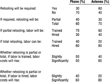
FIGURE 13-6
3. That the company will have to hire new employees?
4. That labor costs will rise slightly?
5. That labor costs will rise significantly?
BEFORE CONTINUING, CONSTRUCT TWO PROBABILITY TREES AND ANSWER THE FIVE QUESTIONS FOR EACH TREE.
Part 1 of the solution to Exercise 38 (page 335) shows the two probability trees. Part 2 provides the answers to the questions.
Estimating is what we do when we run out of data. The language of estimating is probability, and the laws of probability are the grammar of that language.
Probability is one of the most important concepts covered in this book because probability permeates all analysis. Yet it’s one of the least understood concepts and one of the most difficult to deal with effectively because the laws of probability are often counterintuitive.
Proper application of the laws of probability is not something that humans do instinctively.
Despite the trappings of mathematical certainty and scientific objectivity, probability is driven much more by subjective judgments than by mathematical calculation. These subjective judgments, like all others, are subject to biases and other troublesome human mental traits.
Most people can intuitively see the answer to only the most simple problems involving probability.
We determine probability in basically two ways: by computation, when we have the requisite data, and by frequency and experience, when we don’t.
The two types of probability we encounter most often in analysis are mutually exclusive (the “or” type, where we add probabilities) and conditionally dependent (the “and” type, where we multiply them).
When trying to assess the probability of two or more outcomes without a sound basis for judging which is more likely, we should invoke Laplace and assume the probability is equal for all outcomes. We rarely, however, lack a basis for judging likelihood.
We diagram probability outcomes in probability trees, whose construction should follow three rules: the events depicted must be mutually exclusive (meaning each event is distinctive); they must be collectively exhaustive (meaning the tree covers all possible outcomes); and the probabilities at each node (each branching of the tree) must equal 1.0.
Because we humans have widely differing interpretations of adjectival expressions of probability, communicating probability judgments without using numerical percentiles is extremely difficult. There is no easy or right way to do it. But percentiles should be used sparingly and with great care in final reports, because percentiles imply a high degree of analytic precision, which is usually lacking.

