 BEFORE CONTINUING, CONVERT THE TREES INTO A UTILITY MATRIX.
A matrix offers two important advantages over a tree for performing utility analysis. First, the relative differences in utility values of outcomes are more easily perceived in a matrix than in a tree. Second, arithmetic calculations are easier to perform. This is due, in part, to the different configurations of the two structuring devices: a tree is busy, sort of sprawls out, and is sometimes unsymmetrical, while a matrix is a compact, tightly organized, symmetrical unit. Also, the focus of a utility matrix is squarely on alternative outcomes, while a tree portrays whole scenarios in which outcomes are only a part. Depicting scenarios—the strong suit of trees—tends to overshadow and divert attention from the outcomes.
Which is a better vehicle for utility analysis: a matrix or a tree? Naturally, the answer depends on the nature of the problem being analyzed and on the personal preference of the analyst. The analytic steps are the same in either case: construct a matrix or a tree, enter the options and outcomes, define the analytic perspective, assign utility values, assign probabilities, compute expected values, and determine the rankings.
Because it facilitates arithmetic operations, however, a matrix is more suitable than a tree for analyzing a problem from different perspectives and with different classes of outcomes. I address these complexities in the next two chapters.
For now, let me demonstrate how a utility matrix works. Figure 15-1 shows the basic elements of a utility matrix.
The analytic perspective is given in the upper left-hand corner. Options are listed down the left. The class of outcomes is entered above the outcome columns. Each option-outcome combination is represented by a cell. We enter in the cell the utility values and probabilities of that combination and compute its expected value. We then add the expected values for each option and enter the sums in the “Total EV” column, indicating the ranking in the last column.
You can see this more clearly as I convert into a matrix the three utility trees (Figure 15-2) we constructed for the “Japanese Goods” problem in Chapter 14. The resulting matrix is shown in Figure 15-3.
Observe how the matrix does, indeed, focus your attention on the outcomes, placing all the numerical data for each option-outcome combination neatly into a single cell. I find it easier to discern patterns, differences, and similarities with a matrix than with trees, but it’s really a matter of personal preference.
To get a feel for what makes up a utility matrix, try your hand at converting the trees (Figure 15-4) we constructed for the “Egg-Laying Hens” exercise in Chapter 14.
BEFORE CONTINUING, CONVERT THE TREES INTO A UTILITY MATRIX.
Figure 15-5 is the utility matrix for the “Egg-Laying Hens” problem.
Now convert to a matrix the utility trees for the “Jelly Beans” problem (Figure 15-6).
BEFORE CONTINUING, CONVERT THE TREES INTO A UTILITY MATRIX.
FIGURE 15-1 Utility Matrix

FIGURE 15-2
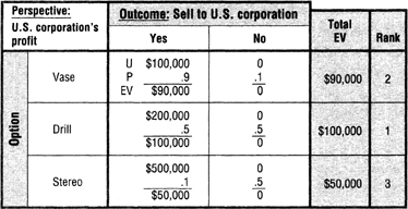
FIGURE 15-3
Figure 15-7 is the utility matrix for the “Jelly Beans” problem.
Convert the trees for the “Securities Investment” problem (Figure 15-8).
BEFORE CONTINUING, CONVERT THE TREES INTO A UTILITY MATRIX.
Figure 15-9 is the utility matrix for the “Securities Investment” problem. “National political and economic situation” is the class of outcome.
Step 1: Identify the options and outcomes to be analyzed.
Step 2: Identify the perspective of the analysis.
Step 3: Construct a utility matrix.
Step 4: Assign a utility value of 0 to 100 (unless dollars are used) to each option-outcome combination—each cell of the matrix—by asking the Utility Question: If we select this option, and this outcome occurs, what is the utility from the perspective of …? There must be at least one 100 unless dollars are used.
Step 5: Assign a probability to each outcome. Determine or estimate this probability by asking the Probability Question: If this option is selected, what is the probability this outcome will occur? The probabilities of all outcomes for a single option must add up to 1.0.
Step 6: Determine the expected values by multiplying each utility by its probability and then adding the expected values for each option.
Step 7: Determine the ranking of the alternative options.
Step 8: Perform a sanity check.
Apply these eight steps in analyzing the “Weather Forecaster’s Dilemma” (Exercise 15), which we encountered in Chapter 8. Here are the particulars again.
FIGURE 15-4

FIGURE 15-5

FIGURE 15-6
FIGURE 15-7

FIGURE 15-8
FIGURE 15-9
Pretend you are the weatherperson on a local TV station. There is a 1 percent chance of snow tomorrow, which is a normal midweek workday. Determine, using a utility matrix, which of two predictions—“Snow” or “Not snow”—is in your better all-around interest. Consider only two outcomes: it snows, and it doesn’t snow.
BEFORE CONTINUING, WORK THE PROBLEM USING A UTILITY MATRIX.
The solution to Exercise 43 (page 338) shows my matrix.
I gave Predict snow-Snow a utility of 100, because most people work and, though they despise how snow delays their commute or hinders their errands and deliveries, they are relieved at having been given fair warning. This is, I believe, the best cell in the matrix for the forecaster because it boosts his or her credibility and enables people to be prepared for the snow, and for that they are grateful.
The worst cell is Predict not snow-Snow. I gave that cell a utility of zero. What could be worse for a weather forecaster?
I gave Predict snow-Not snow a utility of 80. People will have been prepared for snow and be relieved that there was none. Their relief will offset the forecaster’s loss of credibility, unless the forecaster gets the reputation of crying “wolf.”
I gave Predict not snow-Not snow a utility of 30 because, even though working people are pleased that there’s no snow, it’s a nonhappening.
The probabilities were given: .1 probability for snow and, logically, .9 for not snow.
I multiplied the utilities by the probabilities to calculate the expected values. I added the expected values and determined the ranking. My assessment ranks “Predict snow” as the strongly preferred option. (This analysis may explain why weather forecasters on TV and radio tend to predict snow at the very first sign. They’re afraid of ending up in the lower left-hand cell.)
Try the “Weather Forecaster’s Dilemma” exercise at a party some time. I guarantee the discussion of what each cell’s utility should be will liven things up.
In the last exercise in this chapter, to challenge your understanding of how to perform utility analysis, I want you to analyze a problem first with utility trees and then with a matrix.
A group of terrorists has commandeered an airliner to force release of several comrades imprisoned in a foreign capital. You are the commander of a counterterrorist unit. Your supervisor has directed you to determine whether an armed assault on the aircraft should be attempted to save the passengers and crew.
You have carefully analyzed the situation and estimate that, should a rescue be attempted, there is a .1 probability that all passengers and crew will be killed; a .8 probability that only some will be killed; a .1 probability that none will be killed; a 0 probability that, if all are killed, comrades will be released; and a .1 probability that comrades will be released if some or none of the passengers and crew are killed. You have further estimated that, if a rescue is not attempted, there is a .9 probability that comrades will be released.
Part 1: Applying the eight steps of utility-tree analysis (and assigning your own utilities), determine whether a rescue attempt is advisable.
Part 2: Convert and merge the utility trees into a single utility matrix.
BEFORE CONTINUING, WORK THE PROBLEM USING UTILITY-TREE ANALYSIS. THEN CONVERT THE TREES “INTO A UTILITY MATRIX
Part 1 of the solution to Exercise 44 (page 339) shows my version of the completed utility trees. Part 2 of the solution shows my version of the matrix. According to my analysis, a rescue attempt is preferred as its total expected value is nearly twice that of no rescue attempt.


