The concept of probability plays an important role in our daily lives. Assume you have an opportunity to invest some money in a software company. Suppose you know that the company’s records indicate that in the past five years, its profits have been consistently decreasing. Would you still invest your money in it? Do you think the chances are good for the company in the future?
Here is another illustration. Suppose that you are playing a game that involves tossing a single die. Assume that you have already tossed it 10 times, and every time the outcome was the same, a 2. What is your prediction of the eleventh toss? Would you be willing to bet $100 that you will not get a 2 on the next toss? Do you think the die is loaded?
Notice that the decision concerning a successful investment in the software company and the decision of whether or not to bet $100 on the next outcome of the die are both based on probabilities of certain sample results. Namely, the software company’s profits have been declining for the past five years, and the outcome of rolling a 2 ten times in a row seems strange. From these sample results, we might conclude that we are not going to invest our money in the software company or bet on this die. In this lesson, you will learn mathematical ideas and tools that can help you understand such situations.
An event is something that occurs, or happens. For example, flipping a coin is an event, and so is walking in the park and passing by a bench. Anything that could possibly happen is an event.
Every event has one or more possible outcomes. While tossing a coin is an event, getting tails is the outcome of that event. Likewise, while walking in the park is an event, finding your friend sitting on the bench is an outcome of that event.
Suppose a coin is tossed once. There are two possible outcomes, either heads, ![]() , or tails,
, or tails, ![]() . Notice that if the experiment is conducted only once, you will observe only one of the two possible outcomes. An experiment is the process of taking a measurement or making an observation. These individual outcomes for an experiment are each called simple events.
. Notice that if the experiment is conducted only once, you will observe only one of the two possible outcomes. An experiment is the process of taking a measurement or making an observation. These individual outcomes for an experiment are each called simple events.
Example: A die has six possible outcomes: 1, 2, 3, 4, 5, or 6. When we toss it once, only one of the six outcomes of this experiment will occur. The one that does occur is called a simple event.
Example: Suppose that two pennies are tossed simultaneously. We could have both pennies land heads up (which we write as ![]() ), or the first penny could land heads up and the second one tails up (which we write as
), or the first penny could land heads up and the second one tails up (which we write as ![]() ), etc. We will see that there are four possible outcomes for each toss, which are
), etc. We will see that there are four possible outcomes for each toss, which are ![]() , and
, and ![]() . The table below shows all the possible outcomes.
. The table below shows all the possible outcomes.

Figure: The possible outcomes of flipping two coins.
What we have accomplished so far is a listing of all the possible simple events of an experiment. This collection is called the sample space of the experiment.
The sample space is the set of all possible outcomes of an experiment, or the collection of all the possible simple events of an experiment. We will denote a sample space by ![]() .
.
Example: We want to determine the sample space of throwing a die and the sample space of tossing a coin.
Solution: As we know, there are 6 possible outcomes for throwing a die. We may get 1, 2, 3, 4, 5, or 6, so we write the sample space as the set of all possible outcomes:
![]()
Similarly, the sample space of tossing a coin is either heads, ![]() , or tails,
, or tails, ![]() , so we write
, so we write ![]() .
.
Example: Suppose a box contains three balls, one red, one blue, and one white. One ball is selected, its color is observed, and then the ball is placed back in the box. The balls are scrambled, and again, a ball is selected and its color is observed. What is the sample space of the experiment?
It is probably best if we draw a tree diagram to illustrate all the possible selections.
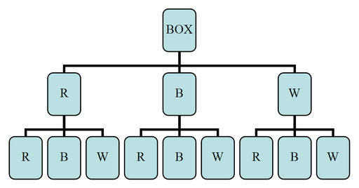
As you can see from the tree diagram, it is possible that you will get the red ball, ![]() , on the first drawing and then another red one on the second,
, on the first drawing and then another red one on the second, ![]() . You can also get a red one on the first and a blue on the second, and so on. From the tree diagram above, we can see that the sample space is as follows:
. You can also get a red one on the first and a blue on the second, and so on. From the tree diagram above, we can see that the sample space is as follows:
![]()
Each pair in the set above gives the first and second drawings, respectively. That is, ![]() is different from
is different from ![]() .
.
We can also represent all the possible drawings by a table or a matrix:

Figure: Table representing the possible outcomes diagrammed in the previous figure. The first column represents the first drawing, and the first row represents the second drawing.
Example: Consider the same experiment as in the last example. This time we will draw one ball and record its color, but we will not place it back into the box. We will then select another ball from the box and record its color. What is the sample space in this case?
Solution: The tree diagram below illustrates this case:

You can clearly see that when we draw, say, a red ball, the blue and white balls will remain. So on the second selection, we will either get a blue or a while ball. The sample space in this case is as shown:
![]()
Now let us return to the concept of probability and relate it to the concepts of sample space and simple events. If you toss a fair coin, the chance of getting tails, ![]() , is the same as the chance of getting heads,
, is the same as the chance of getting heads, ![]() . Thus, we say that the probability of observing heads is 0.5, and the probability of observing tails is also 0.5. The probability,
. Thus, we say that the probability of observing heads is 0.5, and the probability of observing tails is also 0.5. The probability, ![]() , of an outcome,
, of an outcome, ![]() , always falls somewhere between two extremes: 0, which means the outcome is an impossible event, and 1, which means the outcome is guaranteed to happen. Most outcomes have probabilities somewhere in-between.
, always falls somewhere between two extremes: 0, which means the outcome is an impossible event, and 1, which means the outcome is guaranteed to happen. Most outcomes have probabilities somewhere in-between.
Property 1: ![]() , for any event,
, for any event, ![]() .
.
The probability of an event, ![]() , ranges from 0 (impossible) to 1 (certain).
, ranges from 0 (impossible) to 1 (certain).
In addition, the probabilities of all possible simple outcomes of an event must add up to 1. This 1 represents certainty that one of the outcomes must happen. For example, tossing a coin will produce either heads or tails. Each of these two outcomes has a probability of 0.5. This means that the total probability of the coin landing either heads or tails is ![]() That is, we know that if we toss a coin, we are certain to get heads or tails.
That is, we know that if we toss a coin, we are certain to get heads or tails.
Property 2: ![]() when summed over all possible simple outcomes.
when summed over all possible simple outcomes.
The sum of the probabilities of all possible outcomes must add up to 1.
Notice that tossing a coin or throwing a die results in outcomes that are all equally probable. That is, each outcome has the same probability as all the other outcomes in the same sample space. Getting heads or tails when tossing a coin produces an equal probability for each outcome, 0.5. Throwing a die has 6 possible outcomes, each also having the same probability, ![]() . We refer to this kind of probability as classical probability. Classical probability is defined to be the ratio of the number of cases favorable to an event to the number of all outcomes possible, where each of the outcomes is equally likely.
. We refer to this kind of probability as classical probability. Classical probability is defined to be the ratio of the number of cases favorable to an event to the number of all outcomes possible, where each of the outcomes is equally likely.
Probability is usually denoted by ![]() , and the respective elements of the sample space (the outcomes) are denoted by
, and the respective elements of the sample space (the outcomes) are denoted by ![]() etc. The mathematical notation that indicates the probability that an outcome,
etc. The mathematical notation that indicates the probability that an outcome, ![]() , happens is
, happens is ![]() . We use the following formula to calculate the probability of an outcome occurring:
. We use the following formula to calculate the probability of an outcome occurring:
![]()
Example: When tossing two coins, what is the probability of getting a head on both coins, ![]() ? Is the probability classical?
? Is the probability classical?
Since there are 4 elements (outcomes) in the sample space set, ![]() , its size is 4. Furthermore, there is only 1
, its size is 4. Furthermore, there is only 1 ![]() outcome that can occur. Therefore, using the formula above, we can calculate the probability as shown:
outcome that can occur. Therefore, using the formula above, we can calculate the probability as shown:
![]()
Notice that each of the 4 possible outcomes is equally likely. The probability of each is 0.25. Also notice that the total probability of all possible outcomes in the sample space is 1.
Example: What is the probability of throwing a die and getting ![]() ?
?
There are 6 possible outcomes when you toss a die. Thus, the total number of outcomes in the sample space is 6. The event we are interested in is getting a 2, 3, or 4, and there are three ways for this event to occur.
![]()
Therefore, there is a probability of 0.5 that we will get 2, 3, or 4.
Example: Consider tossing two coins. Assume the coins are not balanced. The design of the coins is such that they produce the probabilities shown in the table below:
Table 3.1
| Outcome | Probability |
|
|
|
|
|
|
|
|
|
|
|
|
Figure: Probability table for flipping two weighted coins.
What is the probability of observing exactly one head, and what is the probability of observing at least one head?
Notice that the simple events ![]() and
and ![]() each contain only one head. Thus, we can easily calculate the probability of observing exactly one head by simply adding the probabilities of the two simple events:
each contain only one head. Thus, we can easily calculate the probability of observing exactly one head by simply adding the probabilities of the two simple events:

Similarly, the probability of observing at least one head is:

An event is something that occurs, or happens, with one or more possible outcomes.
An experiment is the process of taking a measurement or making an observation.
A simple event is the simplest outcome of an experiment.
The sample space is the set of all possible outcomes of an experiment, typically denoted by ![]() .
.
For a description of how to find an event given a sample space (1.0), see teachertubemath, Probability Events (2:23).
(i) A ![]() on the die and
on the die and ![]() on the coin
on the coin
(ii) An even number on the die and ![]() on the coin
on the coin
(iii) An even number on the die
(iv) ![]() on the coin
on the coin
are:

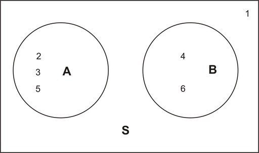
(i) Drawing 2 blue marbles
(ii) Drawing 1 red marble and 1 blue marble
(iii) Drawing 2 red marbles
In this lesson, you will learn how to combine two or more events by finding the union of the two events or the intersection of the two events. You will also learn how to calculate probabilities related to unions and intersections.
Sometimes we need to combine two or more events into one compound event. This compound event can be formed in two ways.
The union of events ![]() and
and ![]() occurs if either event
occurs if either event ![]() , event
, event ![]() , or both occur in a single performance of an experiment. We denote the union of the two events by the symbol
, or both occur in a single performance of an experiment. We denote the union of the two events by the symbol ![]() . You read this as either “
. You read this as either “![]() union
union ![]() ” or “
” or “![]() or
or ![]() .”
.” ![]() means everything that is in set
means everything that is in set ![]() or in set
or in set ![]() or in both sets.
or in both sets.
The intersection of events ![]() and
and ![]() occurs if both event
occurs if both event ![]() and event
and event ![]() occur in a single performance of an experiment. It is where the two events overlap. We denote the intersection of two events by the symbol
occur in a single performance of an experiment. It is where the two events overlap. We denote the intersection of two events by the symbol ![]() . You read this as either “
. You read this as either “![]() intersection
intersection ![]() ” or “
” or “![]() and
and ![]() .”
.” ![]() means everything that is in set
means everything that is in set ![]() and in set
and in set ![]() . That is, when looking at the intersection of two sets, we are looking for where the sets overlap.
. That is, when looking at the intersection of two sets, we are looking for where the sets overlap.
Example: Consider the throw of a die experiment. Assume we define the following events:
![]()
![]()
The sample space of a fair die is ![]() , and the sample spaces of the events
, and the sample spaces of the events ![]() and
and ![]() above are
above are ![]() and
and ![]() .
.
1. An observation on a single toss of the die is an element of the union of ![]() and
and ![]() if it is either an even number, a number that is less than or equal to 3, or a number that is both even and less than or equal to 3. In other words, the simple events of
if it is either an even number, a number that is less than or equal to 3, or a number that is both even and less than or equal to 3. In other words, the simple events of ![]() are those for which
are those for which ![]() occurs,
occurs, ![]() occurs, or both occur:
occurs, or both occur:
![]()
2. An observation on a single toss of the die is an element of the intersection of ![]() and
and ![]() if it is a number that is both even and less than 3. In other words, the simple events of
if it is a number that is both even and less than 3. In other words, the simple events of ![]() are those for which both
are those for which both ![]() and
and ![]() occur:
occur:
![]()
3. Remember, the probability of an event is the sum of the probabilities of its simple events. This is shown for ![]() as follows:
as follows:

Similarly, this can also be shown for ![]() :
:
![]()
Intersections and unions can also be defined for more than two events. For example, ![]() represents the union of three events.
represents the union of three events.
Example: Refer to the above example and answer the following questions based on the definitions of the new events ![]() and
and ![]() .
.
![]()
![]()
1. Since ![]() .
.
2. Since ![]() ,
,
where ![]() is the empty set. This means that there are no elements in the set
is the empty set. This means that there are no elements in the set ![]() .
.
3. Here, we need to be a little careful. We need to find the intersection of the three sets. To do so, it is a good idea to use the associative property by first finding the intersection of sets ![]() and
and ![]() and then intersecting the resulting set with
and then intersecting the resulting set with ![]() .
.
![]()
Again, we get the empty set.
The union of the two events ![]() and
and ![]() , written
, written ![]() , occurs if either event
, occurs if either event ![]() , event
, event ![]() , or both occur on a single performance of an experiment. A union is an 'or' relationship.
, or both occur on a single performance of an experiment. A union is an 'or' relationship.
The intersection of the two events ![]() and
and ![]() , written
, written ![]() , occurs only if both event
, occurs only if both event ![]() and event
and event ![]() occur on a single performance of an experiment. An intersection is an 'and' relationship. Intersections and unions can be used to combine more than two events.
occur on a single performance of an experiment. An intersection is an 'and' relationship. Intersections and unions can be used to combine more than two events.
In this lesson, you will learn what is meant by the complement of an event, and you will be introduced to the Complement Rule. You will also learn how to calculate probabilities when the complement of an event is involved.
The complement ![]() of the event
of the event ![]() consists of all elements of the sample space that are not in
consists of all elements of the sample space that are not in ![]() .
.
Example: Let us refer back to the experiment of throwing one die. As you know, the sample space of a fair die is ![]() . If we define the event
. If we define the event ![]() as observing an odd number, then
as observing an odd number, then ![]() . The complement of
. The complement of ![]() will be all the elements of the sample space that are not in
will be all the elements of the sample space that are not in ![]() . Thus,
. Thus, ![]()
A Venn diagram that illustrates the relationship between ![]() and
and ![]() is shown below:
is shown below:
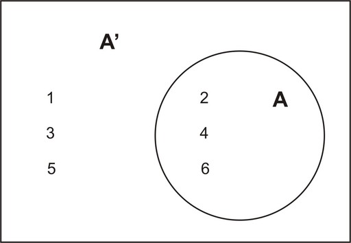
This leads us to say that the sum of the possible outcomes for event ![]() and the possible outcomes for its complement,
and the possible outcomes for its complement, ![]() , is all the possible outcomes in the sample space of the experiment. Therefore, the probabilities of an event and its complement must sum to 1.
, is all the possible outcomes in the sample space of the experiment. Therefore, the probabilities of an event and its complement must sum to 1.
The Complement Rule states that the sum of the probabilities of an event and its complement must equal 1.
![]()
As you will see in the following examples, it is sometimes easier to calculate the probability of the complement of an event than it is to calculate the probability of the event itself. Once this is done, the probability of the event, ![]() , is calculated using the relationship
, is calculated using the relationship ![]() .
.
Example: Suppose you know that the probability of getting the flu this winter is 0.43. What is the probability that you will not get the flu?
Let the event ![]() be getting the flu this winter. We are given
be getting the flu this winter. We are given ![]() . The event not getting the flu is
. The event not getting the flu is ![]() . Thus,
. Thus, ![]() .
.
Example: Two coins are tossed simultaneously. Let the event ![]() be observing at least one head.
be observing at least one head.
What is the complement of ![]() , and how would you calculate the probability of
, and how would you calculate the probability of ![]() by using the Complement Rule?
by using the Complement Rule?
Since the sample space of event ![]() , the complement of
, the complement of ![]() will be all events in the sample space that are not in
will be all events in the sample space that are not in ![]() . In other words, the complement will be all the events in the sample space that do not involve heads. That is,
. In other words, the complement will be all the events in the sample space that do not involve heads. That is, ![]() .
.
We can draw a simple Venn diagram that shows ![]() and
and ![]() when tossing two coins as follows:
when tossing two coins as follows:
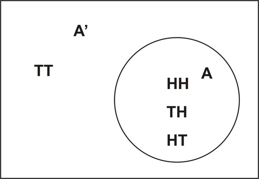
The second part of the problem is to calculate the probability of ![]() using the Complement Rule. Recall that
using the Complement Rule. Recall that ![]() . This means that by calculating
. This means that by calculating ![]() , we can easily calculate
, we can easily calculate ![]() by subtracting
by subtracting ![]() from 1.
from 1.

Obviously, we would have gotten the same result if we had calculated the probability of event ![]() occurring directly. The next example, however, will show you that sometimes it is much easier to use the Complement Rule to find the answer that we are seeking.
occurring directly. The next example, however, will show you that sometimes it is much easier to use the Complement Rule to find the answer that we are seeking.
Example: Consider the experiment of tossing a coin ten times. What is the probability that we will observe at least one head?
What are the simple events of this experiment? As you can imagine, there are many simple events, and it would take a very long time to list them. One simple event may be ![]() , another may be
, another may be ![]() , and so on. There are, in fact,
, and so on. There are, in fact, ![]() ways to observe at least one head in ten tosses of a coin.
ways to observe at least one head in ten tosses of a coin.
To calculate the probability, it's necessary to keep in mind that each time we toss the coin, the chance is the same for heads as it is for tails. Therefore, we can say that each simple event among the 1024 possible events is equally likely to occur. Thus, the probability of any one of these events is ![]() .
.
We are being asked to calculate the probability that we will observe at least one head. You will probably find it difficult to calculate, since heads will almost always occur at least once during 10 consecutive tosses. However, if we determine the probability of the complement of ![]() (i.e., the probability that no heads will be observed), our answer will become a lot easier to calculate. The complement of
(i.e., the probability that no heads will be observed), our answer will become a lot easier to calculate. The complement of ![]() contains only one event:
contains only one event: ![]() . This is the only event in which no heads appear, and since all simple events are equally likely,
. This is the only event in which no heads appear, and since all simple events are equally likely, ![]() .
.
Using the Complement Rule, ![]() .
.
That is a very high percentage chance of observing at least one head in ten tosses of a coin.
The complement ![]() of the event
of the event ![]() consists of all outcomes in the sample space that are not in event
consists of all outcomes in the sample space that are not in event ![]() .
.
The Complement Rule states that the sum of the probabilities of an event and its complement must equal 1, or for the event ![]() .
.
For an explanation of complements and using them to calculate probabilities (1.0), see jsnider3675, An Event's Complement (9:40).
![]()
![]()
![]() .
.
Find each of the following: ![]() .
.
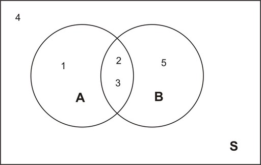
In this lesson, you will learn about the concept of conditional probability and be presented with some examples of how conditional probability is used in the real world. You will also learn the appropriate notation associated with conditional probability.
We know that the probability of observing an even number on a throw of a die is 0.5. Let the event of observing an even number be event ![]() . Now suppose that we throw the die, and we know that the result is a number that is 3 or less. Call this event
. Now suppose that we throw the die, and we know that the result is a number that is 3 or less. Call this event ![]() . Would the probability of observing an even number on that particular throw still be 0.5? The answer is no, because with the introduction of event
. Would the probability of observing an even number on that particular throw still be 0.5? The answer is no, because with the introduction of event ![]() , we have reduced our sample space from 6 simple events to 3 simple events. In other words, since we have a number that is 3 or less, we now know that we have a 1, 2 or 3. This becomes, in effect, our sample space. Now the probability of observing a 2 is
, we have reduced our sample space from 6 simple events to 3 simple events. In other words, since we have a number that is 3 or less, we now know that we have a 1, 2 or 3. This becomes, in effect, our sample space. Now the probability of observing a 2 is ![]() . With the introduction of a particular condition (event
. With the introduction of a particular condition (event ![]() ), we have changed the probability of a particular outcome. The Venn diagram below shows the reduced sample space for this experiment, given that event
), we have changed the probability of a particular outcome. The Venn diagram below shows the reduced sample space for this experiment, given that event ![]() has occurred:
has occurred:
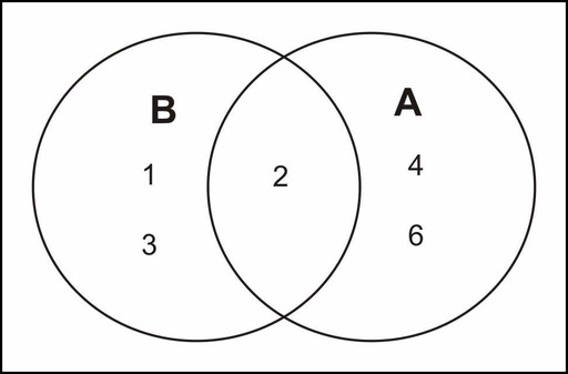
The only even number in the sample space for ![]() is the number 2. We conclude that the probability that
is the number 2. We conclude that the probability that ![]() occurs, given that
occurs, given that ![]() has occurred, is 1:3, or
has occurred, is 1:3, or ![]() . We write this with the notation
. We write this with the notation ![]() , which reads “the probability of
, which reads “the probability of ![]() , given
, given ![]() .” So for the die toss experiment, we would write
.” So for the die toss experiment, we would write ![]() .
.
If ![]() and
and ![]() are two events, then the probability of event
are two events, then the probability of event ![]() occurring, given that event
occurring, given that event ![]() has occurred, is called conditional probability. We write it with the notation
has occurred, is called conditional probability. We write it with the notation ![]() , which reads “the probability of
, which reads “the probability of ![]() , given
, given ![]() .”
.”
To calculate the conditional probability that event ![]() occurs, given that event
occurs, given that event ![]() has occurred, take the ratio of the probability that both
has occurred, take the ratio of the probability that both ![]() and
and ![]() occur to the probability that
occur to the probability that ![]() occurs. That is:
occurs. That is:
![]()
For our example above, the die toss experiment, we proceed as is shown below:
![]()
![]()
To find the conditional probability, we use the formula as follows:
![]()
Example: A medical research center is conducting experiments to examine the relationship between cigarette smoking and cancer in a particular city in the USA. Let ![]() represent an individual who smokes, and let
represent an individual who smokes, and let ![]() represent an individual who develops cancer. This means that
represent an individual who develops cancer. This means that ![]() represents an individual who smokes and develops cancer,
represents an individual who smokes and develops cancer, ![]() represents an individual who smokes but does not develop cancer, and so on. We have four different possibilities, or simple events, and they are shown in the table below, along with their associated probabilities.
represents an individual who smokes but does not develop cancer, and so on. We have four different possibilities, or simple events, and they are shown in the table below, along with their associated probabilities.
Table 3.2
| Simple Events | Probabilities |
|
|
0.10 |
|
|
0.30 |
|
|
0.05 |
|
|
0.55 |
Figure: A table of probabilities for combinations of smoking, ![]() , and developing cancer,
, and developing cancer, ![]() .
.
These simple events can be studied, along with their associated probabilities, to examine the relationship between smoking and cancer.
We have:
![]()
![]()
![]()
![]()
A very powerful way of examining the relationship between cigarette smoking and cancer is to compare the conditional probability that an individual gets cancer, given that he/she smokes, with the conditional probability that an individual gets cancer, given that he/she does not smoke. In other words, we want to compare ![]() with
with ![]() .
.
Recall that ![]() .
.
Before we can use this relationship, we need to calculate the value of the denominator. ![]() is the probability of an individual being a smoker in the city under consideration. To calculate it, remember that the probability of an event is the sum of the probabilities of all its simple events. A person can smoke and have cancer, or a person can smoke and not have cancer. That is:
is the probability of an individual being a smoker in the city under consideration. To calculate it, remember that the probability of an event is the sum of the probabilities of all its simple events. A person can smoke and have cancer, or a person can smoke and not have cancer. That is:
![]()
This tells us that according to this study, the probability of finding a smoker selected at random from the sample space (the city) is 40%. We can continue on with our calculations as follows:
![]()
Similarly, we can calculate the conditional probability of a nonsmoker developing cancer:
![]()
In this calculation, ![]() .
. ![]() can also be found by using the Complement Rule as shown:
can also be found by using the Complement Rule as shown: ![]() .
.
From these calculations, we can clearly see that a relationship exists between smoking and cancer. The probability that a smoker develops cancer is 25%, and the probability that a nonsmoker develops cancer is only 8%. The ratio between the two probabilities is ![]() , which means a smoker is more than three times more likely to develop cancer than a nonsmoker. Keep in mind, though, that it would not be accurate to say that smoking causes cancer. However, our findings do suggest a strong link between smoking and cancer.
, which means a smoker is more than three times more likely to develop cancer than a nonsmoker. Keep in mind, though, that it would not be accurate to say that smoking causes cancer. However, our findings do suggest a strong link between smoking and cancer.
There is another and interesting way to analyze this problem, which has been called the natural frequencies approach (see G. Gigerenzer, “Calculated Risks” Simon and Schuster, 2002).
We will use the probability information given above to demonstrate this approach. Suppose you have 1000 people. Of these 1000 people, 100 smoke and have cancer, and 300 smoke and don’t have cancer. Therefore, of the 400 people who smoke, 100 have cancer. The probability of having cancer, given that you smoke, is ![]() .
.
Of these 1000 people, 50 don’t smoke and have cancer, and 550 don’t smoke and don’t have cancer. Thus, of the 600 people who don’t smoke, 50 have cancer. Therefore, the probability of having cancer, given that you don’t smoke, is ![]() .
.
If ![]() and
and ![]() are two events, then the probability of event
are two events, then the probability of event ![]() occurring, given that event
occurring, given that event ![]() has occurred, is called conditional probability. We write it with the notation
has occurred, is called conditional probability. We write it with the notation ![]() , which reads “the probability of
, which reads “the probability of ![]() , given
, given ![]() .”
.”
Conditional probability can be found with the equation ![]() .
.
Another way to determine a conditional probability is to use the natural frequencies approach.
For an introduction to conditional probability (2.0), see SomaliNew, Conditonal Probability Venn Diagram (4:25).
For an explanation of how to find the probability of "And" statements and dependent events (2.0), see patrickJMT, Calculating Probability - "And" Statements, Dependent Events (5:36).
![]()
![]()
Find ![]() and
and ![]() .
.
![]()
![]()
![]()
Find ![]() and
and ![]() .
.
In this lesson, you will learn how to combine probabilities with the Additive Rule and the Multiplicative Rule. Through the examples in this lesson, it will become clear when to use which rule. You will also be presented with information about mutually exclusive events and independent events.
When the probabilities of certain events are known, we can use these probabilities to calculate the probabilities of their respective unions and intersections. We use two rules, the Additive Rule and the Multiplicative Rule, to find these probabilities. The examples that follow will illustrate how we can do this.
Example: Suppose we have a loaded (unfair) die, and we toss it several times and record the outcomes. We will define the following events:
![]()
![]()
Let us suppose that we have ![]() and
and ![]() . We want to find
. We want to find ![]() .
.
It is probably best to draw a Venn diagram to illustrate this situation. As you can see, the probability of events ![]() or
or ![]() occurring is the union of the individual probabilities of each event.
occurring is the union of the individual probabilities of each event.
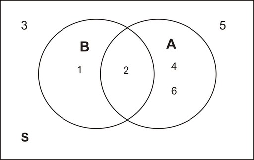
Therefore, adding the probabilities together, we get the following:
![]()
We have also previously determined the probabilities below:

If we add the probabilities ![]() and
and ![]() , we get:
, we get:
![]()
Note that ![]() is included twice. We need to be sure not to double-count this probability. Also note that 2 is in the intersection of
is included twice. We need to be sure not to double-count this probability. Also note that 2 is in the intersection of ![]() and
and ![]() . It is where the two sets overlap. This leads us to the following:
. It is where the two sets overlap. This leads us to the following:
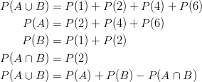
This is the Additive Rule of Probability, which is demonstrated below:
![]()
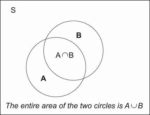
What we have shown is that the probability of the union of two events, ![]() and
and ![]() , can be obtained by adding the individual probabilities,
, can be obtained by adding the individual probabilities, ![]() and
and ![]() , and subtracting the probability of their intersection (or overlap),
, and subtracting the probability of their intersection (or overlap), ![]() . The Venn diagram above illustrates this union.
. The Venn diagram above illustrates this union.
The probability of the union of two events can be obtained by adding the individual probabilities and subtracting the probability of their intersection: ![]() .
.
We can rephrase the definition as follows: The probability that either event ![]() or event
or event ![]() occurs is equal to the probability that event
occurs is equal to the probability that event ![]() occurs plus the probability that event
occurs plus the probability that event ![]() occurs minus the probability that both occur.
occurs minus the probability that both occur.
Example: Consider the experiment of randomly selecting a card from a deck of 52 playing cards. What is the probability that the card selected is either a spade or a face card?
Our event is defined as follows:
![]()
There are 13 spades and 12 face cards, and of the 12 face cards, 3 are spades. Therefore, the number of cards that are either a spade or a face card or both is ![]() That is, event
That is, event ![]() occurs when 1 of 22 cards is selected, the 22 cards being the 13 spade cards and the 9 face cards that are not spade. To find
occurs when 1 of 22 cards is selected, the 22 cards being the 13 spade cards and the 9 face cards that are not spade. To find ![]() , we use the Additive Rule of Probability. First, define two events as follows:
, we use the Additive Rule of Probability. First, define two events as follows:
![]()
![]()
Note that ![]() . Remember, with event
. Remember, with event ![]() , 1 of 13 cards that are spades can be selected, and with event
, 1 of 13 cards that are spades can be selected, and with event ![]() , 1 of 12 face cards can be selected. Event
, 1 of 12 face cards can be selected. Event ![]() occurs when 1 of the 3 face card spades is selected. These cards are the king, jack, and queen of spades. Using the Additive Rule of Probability formula:
occurs when 1 of the 3 face card spades is selected. These cards are the king, jack, and queen of spades. Using the Additive Rule of Probability formula:
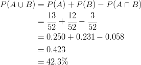
Recall that we are subtracting 0.58 because we do not want to double-count the cards that are at the same time spades and face cards.
Example: If you know that 84.2% of the people arrested in the mid 1990’s were males, 18.3% of those arrested were under the age of 18, and 14.1% were males under the age of 18, what is the probability that a person selected at random from all those arrested is either male or under the age of 18?
First, define the events:
![]()
![]()
Also, keep in mind that the following probabilities have been given to us:
![]()
Therefore, the probability of the person selected being male or under 18 is ![]() and is calculated as follows:
and is calculated as follows:

This means that 88.4% of the people arrested in the mid 1990’s were either male or under 18. If ![]() is empty
is empty ![]() , or, in other words, if there is not overlap between the two sets, we say that
, or, in other words, if there is not overlap between the two sets, we say that ![]() and
and ![]() are mutually exclusive.
are mutually exclusive.
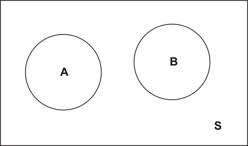
The figure below is a Venn diagram of mutually exclusive events. For example, set ![]() might represent all the outcomes of drawing a card, and set
might represent all the outcomes of drawing a card, and set ![]() might represent all the outcomes of tossing three coins. These two sets have no elements in common.
might represent all the outcomes of tossing three coins. These two sets have no elements in common.
If the events ![]() and
and ![]() are mutually exclusive, then the probability of the union of
are mutually exclusive, then the probability of the union of ![]() and
and ![]() is the sum of the probabilities of
is the sum of the probabilities of ![]() and
and ![]() :
: ![]() .
.
Note that since the two events are mutually exclusive, there is no double-counting.
Example: If two coins are tossed, what is the probability of observing at least one head?
First, define the events as follows:
![]()
![]()
Now the probability of observing at least one head can be calculated as shown:
![]()
Recall from the previous section that conditional probability is used to compute the probability of an event, given that another event has already occurred:
![]()
This can be rewritten as ![]() and is known as the Multiplicative Rule of Probability.
and is known as the Multiplicative Rule of Probability.
The Multiplicative Rule of Probability says that the probability that both ![]() and
and ![]() occur equals the probability that
occur equals the probability that ![]() occurs times the conditional probability that
occurs times the conditional probability that ![]() occurs, given that
occurs, given that ![]() has occurred.
has occurred.
Example: In a certain city in the USA some time ago, 30.7% of all employed female workers were white-collar workers. If 10.3% of all workers employed at the city government were female, what is the probability that a randomly selected employed worker would have been a female white-collar worker?
We first define the following events:
![]()
![]()
We are trying to find the probability of randomly selecting a female worker who is also a white-collar worker. This can be expressed as ![]() .
.
According to the given data, we have:
![]()
Now, using the Multiplicative Rule of Probability, we get:
![]()
Thus, 3.16% of all employed workers were white-collar female workers.
Example: A college class has 42 students of which 17 are male and 25 are female. Suppose the teacher selects two students at random from the class. Assume that the first student who is selected is not returned to the class population. What is the probability that the first student selected is female and the second is male?
Here we can define two events:
![]()
![]()
In this problem, we have a conditional probability situation. We want to determine the probability that the first student selected is female and the second student selected is male. To do so, we apply the Multiplicative Rule:
![]()
Before we use this formula, we need to calculate the probability of randomly selecting a female student from the population. This can be done as follows:
![]()
Now, given that the first student selected is not returned back to the population, the remaining number of students is 41, of which 24 are female and 17 are male.
Thus, the conditional probability that a male student is selected, given that the first student selected was a female, can be calculated as shown below:
![]()
Substituting these values into our equation, we get:
![]()
We conclude that there is a probability of 24.7% that the first student selected is female and the second student selected is male.
Example: Suppose a coin was tossed twice, and the observed face was recorded on each toss. The following events are defined:
![]()
![]()
Does knowing that event ![]() has occurred affect the probability of the occurrence of
has occurred affect the probability of the occurrence of ![]() ?
?
The sample space of this experiment is ![]() , and each of these simple events has a probability of 0.25. So far we know the following information:
, and each of these simple events has a probability of 0.25. So far we know the following information:
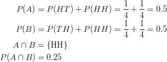
Now, what is the conditional probability? It is as follows:
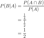
What does this tell us? It tells us that ![]() and also that
and also that ![]() . This means knowing that the first toss resulted in heads does not affect the probability of the second toss being heads. In other words,
. This means knowing that the first toss resulted in heads does not affect the probability of the second toss being heads. In other words, ![]() .
.
When this occurs, we say that events ![]() and
and ![]() are independent events.
are independent events.
If event ![]() is independent of event
is independent of event ![]() , then the occurrence of event
, then the occurrence of event ![]() does not affect the probability of the occurrence of event
does not affect the probability of the occurrence of event ![]() . Therefore, we can write
. Therefore, we can write ![]() .
.
Recall that ![]() . Therefore, if
. Therefore, if ![]() and
and ![]() are independent, the following must be true:
are independent, the following must be true:
![]()
![]()
That is, if two events are independent, ![]() .
.
Example: The table below gives the number of physicists (in thousands) in the US cross-classified by specialty ![]() and base of practice
and base of practice ![]() . (Remark: The numbers are absolutely hypothetical and do not reflect the actual numbers in the three bases.) Suppose a physicist is selected at random. Is the event that the physicist selected is based in academia independent of the event that the physicist selected is a nuclear physicist? In other words, is event
. (Remark: The numbers are absolutely hypothetical and do not reflect the actual numbers in the three bases.) Suppose a physicist is selected at random. Is the event that the physicist selected is based in academia independent of the event that the physicist selected is a nuclear physicist? In other words, is event ![]() independent of event
independent of event ![]() ?
?
Table 3.3
|
Academia |
Industry |
Government |
Total | |
|
General Physics |
10.3 | 72.3 | 11.2 | 93.8 |
|
Semiconductors |
11.4 | 0.82 | 5.2 | 17.42 |
|
Nuclear Physics |
1.25 | 0.32 | 34.3 | 35.87 |
|
Astrophysics |
0.42 | 31.1 | 35.2 | 66.72 |
| Total | 23.37 | 104.54 | 85.9 | 213.81 |
Figure: A table showing the number of physicists in each specialty (thousands). These data are hypothetical.
We need to calculate ![]() and
and ![]() . If these two probabilities are equal, then the two events
. If these two probabilities are equal, then the two events ![]() and
and ![]() are indeed independent. From the table, we find the following:
are indeed independent. From the table, we find the following:
![]()
and
![]()
Thus, ![]() , and so events
, and so events ![]() and
and ![]() are not independent.
are not independent.
Caution! If two events are mutually exclusive (they have no overlap), they are not independent. If you know that events ![]() and
and ![]() do not overlap, then knowing that
do not overlap, then knowing that ![]() has occurred gives you information about
has occurred gives you information about ![]() (specifically that
(specifically that ![]() has not occurred, since there is no overlap between the two events). Therefore,
has not occurred, since there is no overlap between the two events). Therefore, ![]() .
.
The Additive Rule of Probability states that the union of two events can be found by adding the probabilities of each event and subtracting the intersection of the two events, or ![]() .
.
If ![]() contains no simple events, then
contains no simple events, then ![]() and
and ![]() are mutually exclusive. Mathematically, this means
are mutually exclusive. Mathematically, this means ![]() .
.
The Multiplicative Rule of Probability states ![]() .
.
If event ![]() is independent of event
is independent of event ![]() , then the occurrence of event
, then the occurrence of event ![]() does not affect the probability of the occurrence of event
does not affect the probability of the occurrence of event ![]() . Mathematically, this means
. Mathematically, this means ![]() . Another formulation of independence is that if the two events
. Another formulation of independence is that if the two events ![]() and
and ![]() are independent, then
are independent, then ![]() .
.
For an explanation of how to find probabilities using the Multiplicative and Additive Rules with combination notation (1.0), see bullcleo1, Determining Probability (9:42).
For an explanation of how to find the probability of 'and' statements and independent events (1.0), see patrickJMT, Calculating Probability - "And" Statements, Independent Events (8:04).
![]()
Inferential Statistics is a method of statistics that consists of drawing conclusions about a population based on information obtained from samples. Samples are used because it can be quite costly in time and money to study an entire population. In addition, because of the inability to actually reach everyone in a census, a sample can be more accurate than a census.
The most important characteristic of any sample is that it must be a very good representation of the population. It would not make sense to use the average height of basketball players to make an inference about the average height of the entire US population. Likewise, it would not be reasonable to estimate the average income of the entire state of California by sampling the average income of the wealthy residents of Beverly Hills. The goal of sampling is to obtain a representative sample. There are a number of different methods for taking representative samples, and in this lesson, you will learn about simple random samples. You will also be presented with the various counting rules used to calculate probabilities.
A simple random sample of size ![]() is one in which all samples of size
is one in which all samples of size ![]() are equally likely to be selected. In other words, if
are equally likely to be selected. In other words, if ![]() elements are selected from a population in such a way that every set of
elements are selected from a population in such a way that every set of ![]() elements in the population has an equal probability of being selected, then the
elements in the population has an equal probability of being selected, then the ![]() elements form a simple random sample.
elements form a simple random sample.
Example: Suppose you randomly select 4 cards from an ordinary deck of 52 playing cards, and all the cards selected are kings. Would you conclude that the deck is still an ordinary deck, or would you conclude that the deck is not an ordinary one and probably contains more than 4 kings?
The answer depends on how the cards were drawn. It is possible that the 4 kings were intentionally put on top of the deck, and hence, the drawing of the 4 kings was not unusual, and in fact, it was actually certain. However, if the deck was shuffled well, getting 4 kings is highly improbable.
Example: Suppose a lottery consists of 100 tickets, and one winning ticket is to be chosen. What would be a fair method of selecting a winning ticket?
First, we must require that each ticket has an equal chance of winning. That is, each ticket must have a probability of ![]() of being selected. One fair way of doing this is to mix up all the tickets in a container and blindly pick one ticket. This is an example of random sampling.
of being selected. One fair way of doing this is to mix up all the tickets in a container and blindly pick one ticket. This is an example of random sampling.
However, this method would not be too practical if we were dealing with a very large population, such as, say, a million tickets, and we were asked to select 5 winning tickets. One method of picking a simple random sample is to give each element in the population a number. Then use a random number generator to pick 5 numbers. The people who were assigned one of the five numbers would then be the winners.
Some experiments have so many simple events that it is impractical to list them all. Tree diagrams are helpful in determining probabilities in these situations.
Example: Suppose there are six balls in a box. They are identical, except in color. Two balls are red, three are blue, and one is yellow. We will draw one ball, record its color, and then set it aside. Next, we will draw another ball and record its color. With the aid of a tree diagram, calculate the probability of each of the possible outcomes of the experiment.
We first draw a tree diagram to aid us in seeing all the possible outcomes of this experiment.
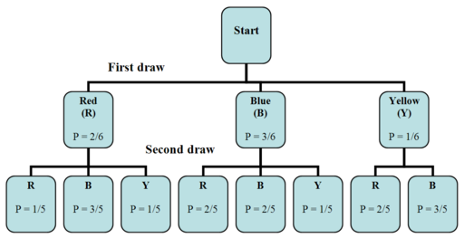
The tree diagram shows us the two stages of drawing two balls without putting the first one back into the box. In the first stage, we pick a ball blindly. Since there are 2 red balls, 3 blue balls, and 1 yellow ball, the probability of getting a red ball is ![]() , the probability of getting a blue ball is
, the probability of getting a blue ball is ![]() , and the probability of getting a yellow ball is
, and the probability of getting a yellow ball is ![]() .
.
Remember that the probability associated with the second ball depends on the color of the first ball. Therefore, the two stages are not independent. To calculate the probabilities when selecting the second ball, we can look back at the tree diagram.
When taking the first ball and the second ball into account, there are eight possible outcomes for the experiment:
![]() : red on the
: red on the ![]() and red on the
and red on the ![]()
![]() : red on the
: red on the ![]() and blue on the
and blue on the ![]()
![]() : red on the
: red on the ![]() and yellow on the
and yellow on the ![]()
![]() : blue on the
: blue on the ![]() and red on the
and red on the ![]()
![]() : blue on the
: blue on the ![]() and blue on the
and blue on the ![]()
![]() : blue on the
: blue on the ![]() and yellow on the
and yellow on the ![]()
![]() : yellow on the
: yellow on the ![]() and red on the
and red on the ![]()
![]() : yellow on the
: yellow on the ![]() and blue on the
and blue on the ![]()
We want to calculate the probability of each of these outcomes. This is done as is shown below.
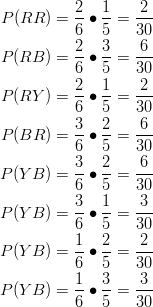
Notice that all of the probabilities add up to 1, as they should.
When using a tree diagram to compute probabilities, you multiply the probabilities as you move along a branch. In the above example, if we are interested in the outcome ![]() , we note that the probability of picking a red ball on the first draw is
, we note that the probability of picking a red ball on the first draw is ![]() . We then go to the second branch, choosing a red ball on the second draw, the probability of which is
. We then go to the second branch, choosing a red ball on the second draw, the probability of which is ![]() . Therefore, the probability of choosing
. Therefore, the probability of choosing ![]() is
is ![]() . The method used to solve the example above can be generalized to any number of stages.
. The method used to solve the example above can be generalized to any number of stages.
Example: A restaurant offers a special dinner menu every day. There are three entrées, five appetizers, and four desserts to choose from. A customer can only select one item from each category. How many different meals can be ordered from the special dinner menu?
Let’s summarize what we have.
Entrees: 3
Appetizer: 5
Dessert: 4
We use the Multiplicative Rule above to calculate the number of different dinners that can be selected. We simply multiply each of the numbers of choices per item together: ![]() . Thus, there are 60 different dinners that can be ordered by the customers.
. Thus, there are 60 different dinners that can be ordered by the customers.
The Multiplicative Rule of Counting states the following:
(I) If there are ![]() possible outcomes for event
possible outcomes for event ![]() and
and ![]() possible outcomes for event
possible outcomes for event ![]() , then there are a total of
, then there are a total of ![]() possible outcomes for event
possible outcomes for event ![]() followed by event
followed by event ![]() .
.
Another way of stating this is as follows:
(II) Suppose you have ![]() sets of elements, with
sets of elements, with ![]() elements in the first set,
elements in the first set, ![]() elements in the second set, and
elements in the second set, and ![]() elements in the
elements in the ![]() set, and you want to take one sample from each of the
set, and you want to take one sample from each of the ![]() sets. The number of different samples that can be formed is the product
sets. The number of different samples that can be formed is the product ![]() .
.
Example: In how many different ways can you seat 8 people at a dinner table?
For the first seat, there are eight choices. For the second, there are seven remaining choices, since one person has already been seated. For the third seat, there are 6 choices, since two people are already seated. By the time we get to the last seat, there is only one seat left. Therefore, using the Multiplicative Rule above, we get ![]() .
.
The multiplication pattern above appears so often in statistics that it has its own name, which is factorial, and its own symbol, which is '!'. When describing it, we say, “Eight factorial,” and we write, "8!."
Factorial Notation
![]()
Example: Suppose there are 30 candidates that are competing for three executive positions. How many different ways can you fill the three positions?
Since there are three executive positions and 30 candidates, let ![]() the number of candidates that are available to fill the first position,
the number of candidates that are available to fill the first position, ![]() the number of candidates remaining to fill the second position, and
the number of candidates remaining to fill the second position, and ![]() the number of candidates remaining to fill the third position.
the number of candidates remaining to fill the third position.
Hence, we have the following:

The number of different ways to fill the three executive positions with the given candidates is ![]() .
.
The arrangement of elements in a distinct order, as the example above shows, is called a permutation. Thus, from the example above, there are 24,360 possible permutations of three elements drawn from a set of 30 elements.
The Counting Rule for Permutations states the following:
The number of ways to arrange ![]() different objects in order within
different objects in order within ![]() positions is
positions is ![]() .
.
Example: Let’s compute the number of ordered seating arrangements we have with 8 people and only 5 seats.
In this case, we are considering a total of ![]() people, and we wish to arrange
people, and we wish to arrange ![]() of these people to be seated. Substituting into the permutation equation, we get the following:
of these people to be seated. Substituting into the permutation equation, we get the following:
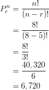
Another way of solving this problem is to use the Multiplicative Rule of Counting. Since there are only 5 seats available for 8 people, for the first seat, there are 8 people available. For the second seat, there are 7 remaining people available, since one person has already been seated. For the third seat, there are 6 people available, since two people have already been seated. For the fourth seat, there are 5 people available, and for the fifth seat, there are 4 people available. After that, we run out of seats. Thus, ![]() .
.
Example: The board of directors at The Orion Foundation has 13 members. Three officers will be elected from the 13 members to hold the positions of a provost, a general director, and a treasurer. How many different slates of three candidates are there if each candidate must specify which office he or she wishes to run for?
Each slate is a list of one person for each of three positions: the provost, the general director, and the treasurer. If, for example, Mr. Smith, Mr. Hale, and Ms. Osborn wish to be on the slate together, there are several different slates possible, depending on which one will run for provost, which one will run for general director, and which one will run for treasurer. This means that we are not just asking for the number of different groups of three names on the slate, but we are also asking for a specific order, since it makes a difference which name is listed in which position.
When computing the answer, ![]() and
and ![]() .
.
Using the permutation formula, we get the following:
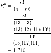
Thus, there are 1,716 different slates of officers possible.
Notice that in our previous examples, the order of people or objects was taken into account. What if the order is not important? For example, in the previous example for electing three officers, what if we wish to choose 3 members of the 13 member board to attend a convention. Here, we are more interested in the group of three, but we are not interested in their order. In other words, we are only concerned with different combinations of 13 people taken 3 at a time. The permutation formula will not work here, since, in this situation, order is not important. However, we have a new formula that will compute different combinations.
The Counting Rule for Combinations states the following:
The number of combinations of ![]() objects taken
objects taken ![]() at a time is
at a time is ![]() .
.
It is important to notice the difference between permutations and combinations. When we consider grouping and order, we use permutations, but when we consider grouping with no particular order, we use combinations.
Example: How many different groups of 3 are possible when taken out of 13 people?
Here, we are interested in combinations of 13 people taken 3 at a time. To find the answer, we can use the combination formula: ![]()
![]()
This means that there are 286 different groups of 3 people to go to the convention.
In the above computation, you can see that the difference between the formulas for ![]() and
and ![]() is the factor
is the factor ![]() in the denominator of the fraction. Since
in the denominator of the fraction. Since ![]() is the number of different orders of
is the number of different orders of ![]() objects, and combinations ignore order, we divide by the number of different orders.
objects, and combinations ignore order, we divide by the number of different orders.
Example: You are taking a philosophy course that requires you to read 5 books out of a list of 10 books. You are free to select any 5 books and read them in whichever order that pleases you. How many different combinations of 5 books are available from a list of 10?
Since consideration of the order in which the books are selected is not important, we compute the number of combinations of 10 books taken 5 at a time. We use the combination formula as is shown below:

This means that there are 252 different groups of 5 books that can be selected from a list of 10 books.
Inferential Statistics is a method of statistics that consists of drawing conclusions about a population based on information obtained from a subset or sample of the population.
A random sampling is a procedure in which each sample of a given size is equally likely to be selected.
The Multiplicative Rule of Counting states that if there are ![]() possible outcomes for event
possible outcomes for event ![]() and
and ![]() possible outcomes for event
possible outcomes for event ![]() , then there are a total of
, then there are a total of ![]() possible outcomes for the series of events
possible outcomes for the series of events ![]() followed by
followed by ![]() .
.
The factorial sign, or ‘!’, is defined as ![]() .
.
The number of permutations (ordered arrangements) of ![]() different objects within
different objects within ![]() positions is
positions is ![]() .
.
The number of combinations (unordered arrangements) of ![]() objects taken
objects taken ![]() at a time is
at a time is ![]() .
.
Technology Note: Generating Random Numbers on the TI-83/84 Calculator
Press [MATH], and then scroll to the right and choose PRB. Next, choose '1:rand' and press [ENTER] twice. The calculator returns a random number between 0 and 1. If you are taking a sample of 100, you need to use the first three digits of the random number that has been returned. If the number is out of range (that is, if the first three digits of the number form a number that is greater than 100), press [ENTER] again, and the calculator will return another random number. Similarly, if a the calculator returns the same first three digits more than once, you can ignore them and press [ENTER] again.
Technology Note: Computing Factorials, Permutations and Combination on the TI-83/84 Calculator
Press [MATH], and then scroll to the right and choose PRB. You will see the following choices, among others: '2:nPr', '3:nCr'. and '4:!'. The screenshots below show the menu and the proper uses of these commands.
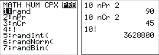
Technology Note: Using EXCEL to Computer Factorials, Permutations and Combinations
In Excel, the commands shown above are entered as follows:
![]() PERMUT(10,2)
PERMUT(10,2)
![]() COMBIN(10,2)
COMBIN(10,2)
 FACT(10)
Keywords
Additive Rule of Probability
Classical probability
Combinations
Complement
Complement Rule
Compound event
Conditional probability
Counting Rule for Combinations
Counting Rule for Permutations
Event
Experiment
Factorial
Independent events
Intersection of events
Multiplicative Rule of Counting
Multiplicative Rule of Probability
Mutually exclusive
Natural frequencies approach
Permutation
Sample space
Simple events
Simple random sample
Tree diagram
Union of events
Venn diagram