For actually running the computational graph, first we will initialize all the variables in our program. The following screenshot shows the lines of code used for running the computational graph:
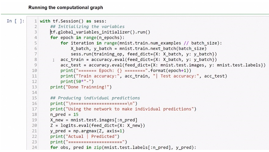
In line 3, we initialize all the variables in our program. Now, here, we don't have any variables explicitly. However, the variables that are inside are fully connected. The fully_connected function is where we have all the hidden layers that contain the weights. These are the variables which is why we must initialize the variables with the global_ variables_initializer object and run this node. For each epoch, we run this loop 20 times. Now, for each iteration that we have in the number of examples over the batch size, which is 80, we get the values for the features and the targets. So this will be 80 data points for each iteration. Then, we run the training operation and will pass as x; we will pass the feature values and here we will pass the target values. Remember, x and y are our placeholders. Then, we evaluate the accuracy of the training and then evaluate the accuracy in the testing dataset, and we get the testing dataset. We get from mnist.test.images, and so these are now the features and test.labels are the targets. Then, we print the two accuracies after these two loops are completed.
We then produce some individual predictions for the first 15 images in the testing dataset. After running this, we get the first epoch, with a training accuracy of 86 percent and a testing accuracy of 88-89 percent. The following screenshot shows the results of training and the testing results for different epochs:

The programs takes a little bit of time to run, but after 20 epochs, the testing accuracy is almost 97 percent. The following screenshot shows the actual labels and the predicted labels. These are the predictions the network made:
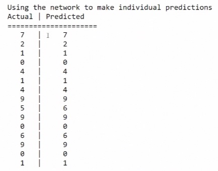
So we have built our first DNN model and we were able to classify handwritten digits using this program with almost 97 percent accuracy.