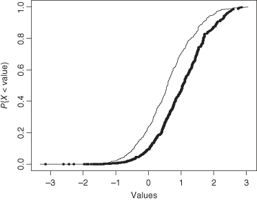
Figure 3.1 Two cumulative distributions F and G that differ by a shift in the median value. The fine line denotes F; the thick line corresponds to G.
Chapter 3
Two Naturally Occurring Probability Distributions
In this chapter, you learn to recognize and describe the binomial and Poisson probability distributions in terms of their cumulative distribution functions and their expectations. You’ll learn when to apply these distributions in your future work along with methods for estimating their parameters using R.
Life constantly calls upon us to make decisions. Should penicillin or erythromycin be prescribed for an infection? Is one brand of erythromycin preferable to another? Which fertilizer should be used to get larger tomatoes? Which style of dress should our company manufacture (i.e., which style will lead to greater sales)?
My wife often asks me what appears to be a very similar question, “which dress do you think I should wear to the party?” But this question is really quite different from the others as it asks what a specific individual, me, thinks about dresses that are to be worn by another specific individual, my wife. All the other questions reference the behavior of a yet-to-be-determined individual selected at random from a population.
Is Alice taller than Peter? It won’t take us long to find out: We just need to put the two back to back or measure them separately.* The somewhat different question, “are girls taller than boys?” is not answered quite so readily. How old are the boys and girls? Generally, but not always, girls are taller than boys until they enter adolescence. Even then, what may be true in general for boys and girls of a specified age group may not be true for a particular girl and a particular boy.
Put in its most general and abstract form, what we are asking is whether a numerical observation X made on an individual drawn at random from one population will be larger than a similar numerical observation Y made on an individual drawn at random from a second population.
Let FW[w] denote the probability that the numerical value of an observation from the distribution W will be less than or equal to w. FW[w] is a monotone nondecreasing function, that is, a graph of FW either rises or remains level as w increases. In symbols, if ε > 0, then 0 = FW[–∞] ≤ FW[w] = Pr{W ≤ w} ≤ Pr{W ≤ w + ε} = FW[w + ε] ≤ FW[∞] = 1.
Two such cumulative distribution functions, Fw and Gw, are depicted in Figure 3.1.
Figure 3.1 Two cumulative distributions F and G that differ by a shift in the median value. The fine line denotes F; the thick line corresponds to G.
Note the following in this figure:
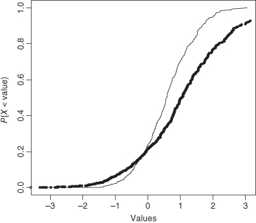
Many treatments act by shifting the distribution of values, as shown in Figure 3.1. The balance of this chapter and the next is concerned with the detection of such treatment effects. The possibility exists that the effects of treatment are more complex than is depicted in Figure 3.1. In such cases, the introductory methods described in this text may not be immediately applicable; see, for example, Figure 3.2, in which the population represented by the thick line is far more variable than the population represented by the thin line.
Figure 3.2 Two cumulative distributions whose mean and variance differ.
Exercise 3.1: Is it possible that an observation drawn at random from the distribution FX depicted in Figure 3.1 could have a value larger than an observation drawn at random from the distribution GX?*
Suppose we’ve collected a sample of n observations X = {x1, x2, … , xn}. The empirical (observed) cumulative distribution function Fn[x] is equal to the number of observations that are less than or equal to x divided by the size of our sample n. If we’ve sorted the sample using the R command sort(X) so that x[1] ≤ x[2] ≤ … ≤ x[n], then the empirical distribution function Fn[x] is
0    if x < x1
k/n  if x lies between x[k] and x[k+1]
1    if x > x[n].
If the observations in the sample all come from the same population distribution F and are independent of one another, then as the sample size n gets larger, Fn will begin to resemble F more and more closely. We illustrate this point in Figure 3.3, with samples of size 10, 100, and 1000 all taken from the same distribution.
Figure 3.3 Three empirical distributions based on samples of size 10 (staircase), 100 (circles), and 1000 independent observations from the same population. The R code needed to generate this figure will be found in Chapter 4.
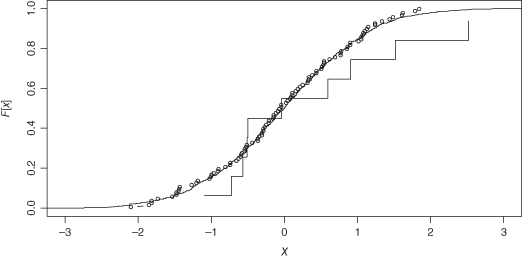
Figure 3.3 reveals what you will find in your own samples in practice: The fit between the empirical (observed) and the theoretical distribution is best in the middle of the distribution near the median and worst in the tails.
We need to distinguish between discrete random observations made when recording the number of events that occur in a given period, from the continuous random observations made when taking measurements.
Discrete random observations usually take only integer values (positive or negative) with nonzero probability. That is,
The cumulative distribution function F[x] is

The expected value of such a distribution is defined as

The binomial and the Poisson are discrete distributions that are routinely encountered in practice.
Exercise 3.2: If X and Y are two independent discrete random variables, show that the expected value of X + Y is equal to the sum of the expected values of X and Y. Hint: Use the knowledge that
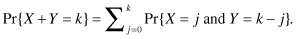
We can also show that the variance of two independent discrete random variables is the sum of their variances.
The binomial distribution arises whenever we perform a series of independent trials each of which can result in either success or failure, and the probability of success is the same for each trial. Survey questions that offer just two alternatives, male or female, smoker or nonsmoker, like or dislike, give rise to binomial distributions.
Recall from the preceding chapter (Section 2.2.3) that when we perform n trials (flip a coin n times, mark n completed survey questions), each with a probability p of success, the probability of observing n successes is given by the following formula:

where  denotes the number of different possible rearrangements of k successes and n – k failures. The cumulative distribution function of a binomial is a step function, equal to zero for all values less than 0 and to one for all values greater than or equal to n.
The expected number of successes in a large number of repetitions of a single binomial trial is p. The expected number of successes in a sufficiently large number of sets of n binomial trials each with a probability p of success is np.
Though it seems obvious that the mean of a sufficiently large number of sets of n binomial trials each with a probability p of success will be equal to np, many things that seem obvious in mathematics aren’t. Besides, if it’s that obvious, we should be able to prove it. Given sufficient familiarity with high school algebra, it shouldn’t be at all difficult.
If a variable X takes a discrete set of values {… , 0,1, … , k, … } with corresponding probabilities {… f0,f1, … , fk, … }, its mean or expected value, written EX, is given by the summation: … + 0f0 + 1f1+ … + kfk + … which we may also write as Σkkfk. For a binomial variable, this sum is
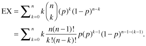
Note that the term on the right is equal to zero when k = 0, so we can start the summation at k = 1. Factoring n and p outside the summation and using the k in the numerator to reduce k! to (k – 1)!, we have
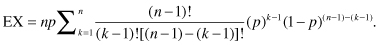
If we change the notation a bit, letting j = (k-1) and m = (n-1), this can be expressed as
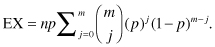
The summation on the right side of the equals sign is of the probabilities associated with all possible outcomes for the binomial random variable B(n, p), so it must be and is equal to 1. Thus, EX = np, a result that agrees with our intuitive feeling that in the long run, the number of successes should be proportional to the probability of success.
Suppose we send out several hundred individuals to interview our customers and find out if they are satisfied with our products. Each individual has the responsibility of interviewing exactly 10 customers. Collating the results, we observe several things:
When we reported these results to our boss, she only seemed interested in the first of them. “Results always vary from interviewer to interviewer, and from sample to sample. And the percentages you reported, apart from the 74% satisfaction rate, are immediate consequences of the binomial distribution.”
Clearly, our boss was familiar with the formula for k successes in n trials given in Section 2.2.3. From our initial finding, she knew that p = 0.74. Thus,

To find the median of this distribution, its 50th percentile, we can use R as follows:
 qbinom(.50,10,0.74)
[1] 7
 qbinom(.50,10,0.74)
[1] 7
To find the proportion of samples with no dissatisfied customers:
 dbinom(10,10,0.74)
[1] 0.0492399
 dbinom(10,10,0.74)
[1] 0.0492399
To find the proportion of samples with four or less satisfied customers:
 pbinom(4,10,0.74)
To display this binomial distribution completely and find its mode:
 #create a vector called binom.vals to hold all the #possible values the results of 10 binomial trials #might take.
  #store 0 to 10 in the vector to binom.vals
 binom.vals = 0:10
 binom.prop = dbinom(binom.vals,10,0.74)
 #display the results
 binom.prop
[1] 1.411671e-06 4.017833e-05 5.145917e-04 3.905619e-03 1.945299e-02
[6] 6.643943e-02 1.575807e-01 2.562851e-01 2.735350e-01 1.730051e-01
[11] 4.923990e-02
The scientific notation used by R in reporting very small or very large values may be difficult to read. Try
 round(binom.prop,3)
for a slightly different view. The 3 asks for three places to the right of the decimal point. Any road, 4.924e-02 is the same as 0.04924.
To find the mode, proceed in two steps
 max(binom.prop)
[1] 2.735350e-01
 max(binom.prop)
[1] 2.735350e-01
The elements of vectors are numbered consecutively beginning at [1]. The mode of the distribution, the outcome with the greatest proportion show above, is located at position 9 in the vector.
 binom.vals[9]
[1] 8
 binom.vals[9]
[1] 8
tells us that the modal outcome is 8 successes.
To find the mean or expected value of this binomial distribution, let us first note that the computation of the arithmetic mean can be simplified when there are a large number of ties by multiplying each distinct number k in a sample by the frequency fk with which it occurs;

We can have only 11 possible outcomes as a result of our interviews: 0, 1, … , or 10 satisfied customers. We know from the binomial distribution the frequency fi with which each outcome may be expected to occur; so that the population mean is given by the formula

For our binomial distribution, we have the values of the variable in the vector binom.vals and their proportions in binom.prop. To find the expected value of our distribution using R, type
 sum(binom.vals*binom.prop)
[1] 7.4
 sum(binom.vals*binom.prop)
[1] 7.4
This result, we notice, is equal to 10*0.74 or 10p. This is not surprising, as we know that the expected value of the binomial distribution is equal to the product of the number of trials and the probability of success at each trial.
Warning: In the preceding example, we assumed that our sample of 1000 customers was large enough that we could use the proportion of successes in that sample, 740 out of 1000 as if it were the true proportion in the entire distribution of customers. Because of the variation inherent in our observations, the true proportion might have been greater or less than our estimate.
Exercise 3.3: Which is more likely: Observing two or more successes in 8 trials with a probability of one-half of observing a success in each trial, or observing three or more successes in 7 trials with a probability of 0.6 of observing a success? Which set of trials has the greater expected number of successes?
Exercise 3.4: Show without using algebra that if X and Y are independent identically distributed binomial variables B(n,p), then X + Y is distributed as B(2n,p).
Unless we have a large number of samples, the observed or empirical distribution may differ radically from the expected or theoretical distribution.
Exercise 3.5: One can use the R function rbinom to generate the results of binomial sampling. For example, binom = rbinom(100,10,0.6) will store the results of 100 binomial samples of 10 trials, each with probability of 0.6 of success in the vector binom. Use R to generate such a vector of sample results and to produce graphs to be used in comparing the resulting empirical distribution with the corresponding theoretical distribution.
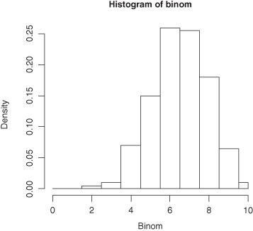
Exercise 3.6: If you use the R code hist(rbinom(200,10,0.65)), the resulting histogram will differ from that depicted in Figure 3.4. Explain why.
Figure 3.4 Histogram, based on 200 trials of B(10,0.65).
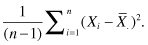
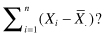
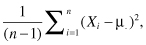
The variance of a sample, a measure of the variation within the sample, is defined as the sum of the squares of the deviations of the individual observations about their mean divided by the sample size minus 1. In symbols, if our observations are labeled X1, X2, up to Xn, and the mean of these observations is written as  , then the variance of our observations is equal to
Both the mean and the variance will vary from sample to sample. If the samples are very large, there will be less variation from sample to sample, and the sample mean and variance will be very close to the mean and variance of the population.
Exercise 3.7: What is the sum of the deviations of the observations from their arithmetic mean? That is, what is
*Exercise 3.8: If you know calculus, use the result of Exercise 3.7 to show that
is minimized if we chose  . In other words, the sum of the squared deviations is a minimum about the mean of a sample.
The problem with using the variance as a measure of dispersion is that if our observations, on temperature, for example, are in degrees Celsius, then the variance would be expressed in square degrees, whatever these are. More often, we report the standard deviation σ, the square root of the variance, as it is in the same units as our observations.
The standard deviation of a sample also provides a measure of its precision.
Exercise 3.9: Recall the classroom data of Chapter 1, classdata = c(141, 156.5, 162, 159, 157, 143.5, 154, 158, 140, 142, 150, 148.5, 138.5, 161, 153, 145, 147, 158.5, 160.5, 167.5, 155, 137). Compute the data’s variance and standard deviation, using the R functions var() and sqrt().
The variance of a binomial variable B(n,p) is np(1 – p). Its standard deviation is  . This formula yields an important property that we will make use of in a latter chapter when we determine how large a sample to take. For if the precision of a sample is proportional to the square root of its sample size, then to make estimates that are twice as precise, we need to take four times as many observations.
The decay of a radioactive element, an appointment to the U.S. Supreme Court, and a cavalry officer kicked by his horse have in common that they are relatively rare but inevitable events. They are inevitable, that is, if there are enough atoms, enough seconds or years in the observation period, and enough horses and momentarily careless men. Their frequency of occurrence has a Poisson distribution.
The number of events in a given interval has the Poisson distribution if
The intervals can be in space or time. For example, if we seed a small number of cells into a Petri dish that is divided into a large number of squares, the distribution of cells per square follows the Poisson. The same appears to be true in the way a large number of masses in the form of galaxies are distributed across a very large universe.
Like the binomial variable, a Poisson variable only takes non-negative integer values. If the number of events X has a Poisson distribution such that we may expect an average of λ events per unit interval, then Pr{X = k} = λke–λ/k! for k = 0, 1,2, … . For the purpose of testing hypotheses concerning λ as discussed in the chapter following, we needn’t keep track of the times or locations at which the various events occur; the number of events k is sufficient.
Exercise 3.10: If we may expect an average of two events per unit interval, what is the probability of no events? Of one event?
Exercise 3.11: Show without using algebra that the sum of a Poisson with the expected value λ1 and a second independent Poisson with the expected value λ2 is also a Poisson with the expected value λ1 + λ2.
John Ross of the Wistar Institute held there were two approaches to biology: the analog and the digital. The analog was served by the scintillation counter: one ground up millions of cells then measured whatever radioactivity was left behind in the stew after centrifugation; the digital was to be found in cloning experiments where any necessary measurements would be done on a cell-by-cell basis.
John was a cloner, and, later, as his student, so was I. We’d start out with 10 million or more cells in a 10-mL flask and try to dilute them down to one cell per mL. We were usually successful in cutting down the numbers to 10,000 or so. Then came the hard part. We’d dilute the cells down a second time by a factor of 1 : 10 and hope we’d end up with 100 cells in the flask. Sometimes we did. Ninety percent of the time, we’d end up with between 90 and 110 cells, just as the Poisson distribution predicted. But just because you cut a mixture in half (or a dozen, or a 100 parts) doesn’t mean you’re going to get equal numbers in each part. It means the probability of getting a particular cell is the same for all the parts. With large numbers of cells, things seem to even out. With small numbers, chance seems to predominate.
Things got worse, when I went to seed the cells into culture dishes. These dishes, made of plastic, had a rectangular grid cut into their bottoms, so they were divided into approximately 100 equal size squares. Dropping 100 cells into the dish meant an average of 1 cell per square. Unfortunately for cloning purposes, this average didn’t mean much. Sometimes, 40% or more of the squares would contain two or more cells. It didn’t take long to figure out why. Planted at random, the cells obey the Poisson distribution in space. An average of one cell per square means
Pr{No cells in a square} = 1*e−1/1 = 0.32
Pr{Exactly one cell in a square} = 1*e−1/1 = 0.32
Pr{Two or more cells in a square} = 1–0.32–0.32 = 0.36.
Two cells was one too many. A clone or colony must begin with a single cell (which subsequently divides several times). I had to dilute the mixture a third time to ensure the percentage of squares that included two or more cells was vanishingly small. Alas, the vast majority of squares were now empty; I was forced to spend hundreds of additional hours peering through the microscope looking for the few squares that did include a clone.
Table 3.1 compares the spatial distribution of superclusters of galaxies with a Poisson distribution that has the same expectation. The fit is not perfect due both to chance and to ambiguities in the identification of distinct superclusters.
Table 3.1 Spatial Distribution of Superclusters of Galaxies

To solve the next two exercises, make use of the R functions for the Poisson similar to those we used in studying the binomial similar including dpois, ppois, qpois, and rpois.
Exercise 3.12: Generate the results of 100 samples from a Poisson distribution with an expected number of two events per interval. Compare the graph of the resulting empirical distribution with that of the corresponding theoretical distribution. Determine the 10th, 50th, and 90th percentiles of the theoretical Poisson distribution.
Exercise 3.13: Show that if Pr{X = k} = λke–λ/k! for k = 0, 1,2, … that is, if X is a Poisson variable, then the expected value of X = ΣkkPr{X = k} = λ.
*Exercise 3.14: Show that the variance of the Poisson distribution is also λ.
Exercise 3.15: In subsequent chapters, we’ll learn how the statistical analysis of trials of a new vaccine is often simplified by assuming that the number of infected individuals follows a Poisson rather than a Binomial distribution. To see how accurate an approximation this might be, compare the cumulative distribution functions of a binomial variable, B(100,0.01) and a Poisson variable, P(1) over the range 0 to 100.
Recently, I had the opportunity to participate in the conduct of a very large-scale clinical study of a new vaccine. I’d not been part of the design team, and when I read over the protocol, I was stunned to learn that the design called for inoculating and examining 100,000 patients! 50,000 with the experimental vaccine, and 50,000 controls with a harmless saline solution.
Why so many? The disease at which the vaccine was aimed was relatively rare. In essence, we would be comparing two Poisson distributions. Suppose we could expect 0.8% or 400 of the controls to contract the disease, and 0.7% or 350 of those vaccinated to contract it. Put another way, if the vaccine was effective, we would expect 400/750th of the patients who contracted the disease to be controls. While if the vaccine was ineffective (no better and no worse than no vaccine at all), we would expect 50% of the patients who contracted the disease to be controls. The problem boils down to a single binomial.
Exercise 3.16: In actuality, only 200 of the controls contracted the disease along with 180 of those who had been vaccinated. What is the probability that such a difference might have occurred by chance alone?
The vast majority of the observations we make are on a continuous scale even if, in practice, we only can make them in discrete increments. For example, a man’s height might actually be 1.835421117 m, but we are not likely to record a value with that degree of accuracy (nor want to). If one’s measuring stick is accurate to the nearest millimeter, then the probability that an individual selected at random will be exactly 2 m tall is really the probability that his or her height will lie between 1.9995 and 2.0004 m. In such a situation, it is more convenient to replace the sum of an arbitrarily small number of quite small probabilities with an integral
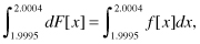
where F[x] is the cumulative distribution function of the continuous variable representing height, and f[x] is its probability density. Note that F[x] is now defined as
As with discrete variables, the cumulative distribution function is monotone nondecreasing from 0 to 1, the distinction being that it is a smooth curve rather than a step function.
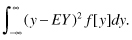
The mathematical expectation of a continuous variable is

and its variance is
The simplest way to obtain continuously distributed random observations is via the same process that gave rise to the Poisson. Recall that a Poisson process is such that events in nonoverlapping intervals are independent and identically distributed. The times† between Poisson events follow an exponential distribution:

When t is zero, exp[–t/λ] is 1 and F[t|λ] is 0. As t increases, exp [–t/λ] decreases rapidly toward zero and F[t|λ] increases rapidly to 1. The rate of increase is inversely proportional to the magnitude of the parameter λ. In fact, log(1 – F[t|λ]) = –t/λ. The next exercise allows you to demonstrate this for yourself.
Exercise 3.17: Draw the cumulative distribution function of an exponentially distributed observation with parameter λ = 3. What is the median? Use the following R code:# using R’s seq() command, divide the interval 0, 12 into increments 1/10th of a unit apart
 t=seq(0,12,0.1)
 F= 1 – exp(-t/3)
 plot (t,F)
*Exercise 3.18: (requires calculus) What is the expected value of an exponentially distributed observation with parameter λ?
The times between counts on a Geiger counter follow an exponential distribution. So do the times between failures of manufactured items, like light bulbs, that rely on a single crucial component.
Exercise 3.19: When you walk into a room, you discover the light in a lamp is burning. Assuming the life of its bulb is exponentially distributed with an expectation of 1 year, how long do you expect it to be before the bulb burns out? (Many people find they get two contradictory answers to this question. If you are one of them, see W. Feller, An Introduction to Probability Theory and Its Applications, 1966, vol. 1, pp. 11–12.)
Most real-life systems (including that complex system known as a human being) have built-in redundancies. Failure can only occur after a series of n breakdowns. If these breakdowns are independent and exponentially distributed, all with the same parameter λ, the probability of failure of the total system at time t > 0 is
In this chapter, we considered the form of three common distributions, two discrete—the binomial and the Poisson, and one continuous—the exponential. You were provided with the R functions necessary to generate random samples, and probability values from the various distributions.
Exercise 3.20: Make a list of all the italicized terms in this chapter. Provide a definition for each one along with an example.
Exercise 3.21: A farmer was scattering seeds in a field so they would be at least a foot apart 90% of the time. On the average, how many seeds should he sow per square foot?
The answer to Exercise 3.1 is yes, of course; an observation or even a sample of observations from one population may be larger than observations from another population even if the vast majority of observations are quite the reverse. This variation from observation to observation is why before a drug is approved for marketing, its effects must be demonstrated in a large number of individuals and not just in one or two. By the same token, when reporting the results of a survey, we should always include the actual frequencies and not just percentages.
Notes
* Quick: Which methods are likely to yield the more accurate comparison? Why?
* If the answer to this exercise is not immediately obvious—you’ll find the correct answer at the end of this chapter—you should reread Chapters 1 and 2 before proceeding further.
* If it’s been a long while or never since you had calculus, note that the differential dx or dy is a meaningless index, so any letter will do, just as Σkfk means exactly the same thing as Σjfj.
† Time is almost but not quite continuous. Modern cosmologists now believe that both time and space are discrete, with time determined only to the nearest 10−23rd of a second, that’s 1/100000000000000000000000th of a second.
