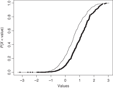
Figure 5.1 The shift to the right of the darker curve represents the potential life-extending effect of treatment with vitamin E.
Chapter 5
Testing Hypotheses
In this chapter, we develop improved methods for testing hypotheses by means of the bootstrap, introduce permutation testing methods, and apply these and the t-test to experiments involving one and two samples. We then address the obvious but essential question: How do we choose the method and the statistic that is best for the problem at hand?
Suppose we were to pot a half-dozen tomato plants in ordinary soil and a second half-dozen plants in soil enriched with fertilizer. If we wait a few months, we can determine whether the addition of fertilizer increases the resulting yield of tomatoes, at least as far as these dozen plants are concerned. But can we extend our findings to all tomatoes? Or, at least, to all tomatoes of the same species that are raised under identical conditions apart from the use of fertilizer.
To ensure that we can extend our findings, we need to proceed as follows: First, the 12 tomato plants used in our study must be a random sample from a nursery. If we choose only plants with especially green leaves for our sample, then our results can be extended only to plants with especially green leaves. Second, we have to divide the 12 plants into two treatment groups at random. If we subdivide by any other method, such as tall plants in one group and short plants in another, then the experiment would not be about fertilizer but about our choices.
I performed just such a randomized experiment a decade or so ago. Only, I was interested in the effects vitamin E might have on the aging of human cells in culture. After several months of abject failure—contaminated cultures, spilled containers—I succeeded in cloning human diploid fibroblasts in eight culture dishes. Four of these dishes were filled with a conventional nutrient solution and four held a potential “life-extending” solution to which vitamin E had been added. All the cells in the dishes came from the same culture so that the initial distribution of cells was completely random.
I waited 3 weeks with my fingers crossed—there is always a risk of contamination with cell cultures—but at the end of this test period, three dishes of each type had survived. I transplanted the cells, let them grow for 24 hours in contact with a radioactive label, and then fixed and stained them before covering them with a photographic emulsion.
Ten days passed and we were ready to examine the autoradiographs. “121, 118, 110, 34, 12, 22.” I read and reread these six numbers over and over again. The larger numbers were indicative of more cell generations and an extended lifespan. If the first three generation-counts were from treated colonies and the last three were from untreated, then I had found the fountain of youth. Otherwise, I really had nothing to report.
How had I reached this conclusion? Let’s take a second, more searching look. First, we identify the primary hypothesis and the alternative hypothesis of interest.
I wanted to assess the life-extending properties of a new experimental treatment with vitamin E. To do this, I had divided my cell cultures at random into two groups: one grown in a standard medium and one grown in a medium containing vitamin E. At the conclusion of the experiment and after the elimination of several contaminated cultures, both groups consisted of three independently treated dishes.
My primary hypothesis was a null hypothesis, that the growth potential of a culture would not be affected by the presence of vitamin E in the media: All the cultures would have equal growth potential. The alternative hypothesis of interest was that cells grown in the presence of vitamin E would be capable of many more cell divisions. This is a one-sided alternative hypothesis.
Under the null hypothesis, the labels “treated” and “untreated” provide no information about the outcomes: The observations are expected to have more or less the same values in each of the two experimental groups. If they do differ, it should only be as a result of some uncontrollable random fluctuations. Thus, if this null or no-difference-among-treatments hypothesis were true, I was free to exchange the treatment labels.
The alternative is a distributional shift like that depicted in Figure 5.1 in which greater numbers of cell generations are to be expected as the result of treatment with vitamin E (though the occasional smaller value cannot be ruled out completely).
Figure 5.1 The shift to the right of the darker curve represents the potential life-extending effect of treatment with vitamin E.
The next step is to choose a test statistic that discriminates between the hypothesis and the alternative. The statistic I chose was the sum of the counts in the group treated with vitamin E. If the alternative hypothesis is true, most of the time this sum ought to be larger than the sum of the counts in the untreated group. If the null hypothesis is true, that is, if it doesn’t make any difference which treatment the cells receive, then the sums of the two groups of observations should be approximately the same. One sum might be smaller or larger than the other by chance, but most of the time the two shouldn’t be all that different.
The third step is to compute the test statistic for each of the possible reassignments of treatment label to result and compare these values with the value of the test statistic as the data were labeled originally. As it happened, the first three observations—121, 118, and 110—were those belonging to the cultures that received vitamin E. The value of the test statistic for the observations as originally labeled is 349 = 121 + 118 + 110.
I began to rearrange (permute) the observations, by randomly reassigning the six labels, three “treated” and three “untreated,” to the six observations. For example: treated, 121 118 34, and untreated, 110 12 22. In this particular rearrangement, the sum of the observations in the first (treated) group is 273. I repeated this step until all  distinct rearrangements had been examined.*
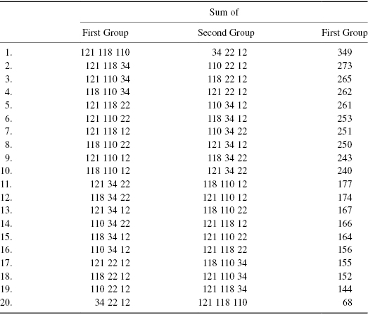
The sum of the observations in the original vitamin E-treated group, 349, is equaled only once and never exceeded in the 20 distinct random relabelings. If chance alone is operating, then such an extreme value is a rare, only a 1-time-in-20 event. If I reject the null hypothesis and embrace the alternative that the treatment is effective and responsible for the observed difference, I only risk making an error and rejecting a true hypothesis once in every 20 times.
In this instance, I did make just such an error. I was never able to replicate the observed life-promoting properties of vitamin E in other repetitions of this experiment. Good statistical methods can reduce and contain the probability of making a bad decision, but they cannot eliminate the possibility.
Exercise 5.1: How was the analysis of the cell culture experiment affected by the loss of two of the cultures due to contamination? Suppose these cultures had escaped contamination and given rise to the observations 90 and 95; what would be the results of a permutation analysis applied to the new, enlarged data set consisting of the following cell counts
Treated 121 118 110 90 Untreated 95 34 22 12?
Hint: To determine how probable an outcome like this is by chance alone, first determine how many possible rearrangements there are. Then list all the rearrangements that are as or more extreme than this one.
In the preceding example, I risked rejecting the null hypothesis in error 5% of the time. Statisticians call this making a Type I error and they call the 5%, the significance level. In fact, I did make such an error, for in future experiments, vitamin E proved to be valueless in extending the life span of human cells in culture.
On the other hand, suppose the null hypothesis had been false, that treatment with vitamin E really did extend life span, and I had failed to reject the null hypothesis. Statisticians call this making a Type II error.
The consequences of each type of error are quite different and depend upon the context of the investigation. Consider the table of possibilities (Table 5.1) arising from an investigation of the possible carcinogenicity of a new headache cure.
Table 5.1 Decision Making Under Uncertainty
| The facts | Investigator’s decision | |
| Not a carcinogen | Compound a carcinogen | |
| Not a carcinogen | Type I error: Manufacturer misses opportunity for profit. | |
| Public denied access to effective treatment. | ||
| Carcinogen | Type II error: Manufacturer sued. | |
| Patients die; families suffer. | ||
We may luck out in that our samples supports the correct hypothesis, but we always run the risk of making either a Type I or a Type II error. We can’t avoid it. If we use a smaller significance level, say 1%, then, if the null hypothesis is false, we are more likely to make a Type II error. If we always accept the null hypothesis, a significance level of 0%, then we guarantee we’ll make a Type II error if the null hypothesis is false. This seems kind of a stupid: why bother to gather data if you’re not going to use the data? But if you read or live Dilbert, then you know this happens all the time.
Exercise 5.2: The nurses have petitioned the CEO of a hospital to allow them to work 12-hour shifts. He wants to please them but is afraid that the frequency of errors may increase as a result of the longer shifts. He decides to conduct a study and to test the null hypothesis that there is no increase in error rate as a result of working longer shifts against the alternative that the frequency of errors increases by at least 30%. Describe the losses associated with Type I and Type II errors.
Exercise 5.3: Design a study. Describe a primary hypothesis of your own along with one or more likely alternatives. The truth or falsity of your chosen hypothesis should have measurable monetary consequences. If you were to test your hypothesis, what would be the consequences of making a Type I error? A Type II error?
Exercise 5.4: Suppose I’m (almost) confident that my candidate will get 60% or more of the votes in the next primary. The alternative that scares me is that she will get 45% or less. To see if my confidence is warranted, I decide to interview 20 people selected at random in a shopping mall and reject my hypothesis if 7 or fewer say they will vote for her.
Exercise 5.5: Individuals were asked to complete an extensive questionnaire concerning their political views and eating preferences. Analyzing the results, a sociologist performed 20 different tests of hypotheses. Unknown to the sociologist, the null hypothesis was true in all 20 cases. What is the probability that the sociologist rejected at least one of the hypotheses at the 5% significance level? (Reread Chapter 2 and Chapter 3 if you are having trouble with this exercise.)
In the previous example, we developed a test of the null hypothesis of no treatment effect against the alternative hypothesis that a positive effect existed. But in many situations, we would also want to know the magnitude of the effect. Does vitamin E extend cell lifespan by 3 cell generations? By 10? By 15?
In Section 1.6.2, we used the bootstrap to obtain estimates of the precision of an estimate of the sample mean or median (or, indeed, any sample percentile). In Section 1.6.2, we showed how to use the bootstrap estimate the precision of the sample mean or median (or, indeed, almost any sample statistic) as an estimator of a population parameter. As a byproduct, we obtain an interval estimate of the corresponding population parameter.
For example, if P05 and P95 are the 5th and 95th percentiles of the bootstrap distribution of the median of the law school LSAT data you used for Exercise 1.13, then the set of values between P05 and P95 provides a 90% confidence interval for the median of the population from which the data were taken.
Exercise 5.6: Obtain an 85% confidence interval for the median of the population from which the LSAT data were taken.
Exercise 5.7: Can this same bootstrap technique be used to obtain a confidence interval for the 90th percentile of the population? For the maximum value in the population?
Suppose we have collected random samples from two populations and want to know the following:
To find out, we would let each sample stand in place of the population from which it is drawn, take a series of bootstrap samples separately from each sample, and compute the difference in means each time.
Suppose our data is stored in two vectors called “control” and “treated.” The R code to obtain the desired interval estimate would be as follows:
 #This program selects 400 bootstrap samples from #your data
 #and then produces an interval estimate of the #difference in population means
 #Record group sizes
 n = length(control)
 m = length(treated)
 #set number of bootstrap samples
 N = 400
 stat = numeric(N)
  #create a vector in which to store the results
 #the elements of this vector will be #numbered from 1 to N
 #Set up a loop to generate a series of bootstrap #samples
 for (i in 1:N){
     #bootstrap sample counterparts are denoted with a "B"
       controlB = sample (control, n, replace = T)
       treatB = sample (treated, m, replace = T)
       stat[i] = mean(treatB) – mean(controlB)
       }
 quantile (x = stat, probs = c(.25,.75))
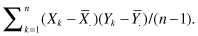
Yet another example of the bootstrap’s application lies in the measurement of the correlation or degree of agreement between two variables. The Pearson correlation of two variables X and Y is defined as the ratio of the covariance between X and Y and the product of the standard deviations of X and Y. The covariance of X and Y is given by the formula
The reason we divide by the product of the standard deviations in assessing the degree of agreement between two variables is that it renders the correlation coefficient free of the units of measurement.
Recall that if X and Y are independent, E(XY) = (EX)(EY), so that the expected value of the covariance and hence the correlation of X and Y is zero. If X and Y increase more or less together as do, for example, the height and weight of individuals, their covariance and their correlation will be positive so that we say that height and weight are positively correlated. I had a boss—more than one, who believed that the more abuse and criticism he heaped on an individual, the more work he could get out of them. Not. Abuse and productivity are negatively correlated; heap on the abuse and work output declines.
If X = –Y, so that the two variables are totally dependent, the correlation coefficient, usually represented in symbols by the Greek letter ρ (rho) will be −1. In all cases, −1 ≤ ρ ≤ 1.
Exercise 5.8: Using the LSAT data from Exercise 1.13 and the bootstrap, obtain an interval estimate for the correlation between the LSAT score and the student’s subsequent GPA. Compare with the result using Pearson correlation, cor.test().
Exercise 5.9: Obtain an interval estimate for the correlation using the bias-corrected and accelerated bootstrap discussed in the previous chapter.
Exercise 5.10: Trying to decide whether to take a trip to Paris or Tokyo, a Canadian student kept track of how many Euros and Yen his dollars would buy. Month by month he found that the values of both currencies were rising. Does this mean that improvements in the European economy are reflected by improvements in the Japanese economy?
Suppose we have derived a 90% confidence interval for some parameter, for example, a confidence interval for the difference in means between two populations, one of which was treated and one that was not. We can use this interval to test the hypothesis that the difference in means is 4 units, by accepting this hypothesis if 4 is included in the confidence interval and rejecting it otherwise. If our alternative hypothesis is nondirectional and two-sided, θA ≠ θB, the test will have a Type I error of 100% − 90% = 10%.
Clearly, hypothesis tests and confidence intervals are intimately related. Suppose we test a series of hypotheses concerning a parameter θ. For example, in the vitamin E experiment, we could test the hypothesis that vitamin E has no effect, θ = 0, or that vitamin E increases life span by 25 generations, θ = 25, or that it increases it by 50 generations, θ = 50. In each case, whenever we accept the hypothesis, the corresponding value of the parameter should be included in the confidence interval.
In this example, we are really performing a series of one-sided tests. Our hypotheses are that θ = 0 against the one-sided alternative that θ > 0, that θ ≤ 25 against the alternative that θ > 25, and so forth. Our corresponding confidence interval will be one-sided also; we will conclude θ < θU if we accept the hypothesis θ = θ0 for all values of θ0 < θU and reject it for all values of θ0 ≥ θU.
Suppose, instead, we’d wanted to make a comparison between two treatments of unknown value or between two proposed direct-mail appeals for funds. Our null hypothesis would be that it didn’t make any difference which treatment or which marketing letter was used; the two would yield equivalent results. Our two-sided alternative would be that one of the two would prove superior to the other. Such a two-sided alternative would lead to a two-sided test in which we would reject our null hypothesis if we observed either very large or very small values of the test statistic. Not surprisingly, one-sided tests lead to one-sided confidence intervals and two-sided tests to two-sided confidence intervals.
Exercise 5.11: What is the relationship between the significance level of a test and the confidence level of the corresponding interval estimate?
Exercise 5.12: In each of the following instances, would you use a one-sided or a two-sided test?
Exercise 5.13: Use the data of Exercise 5.1 to derive an 80% upper confidence bound for the effect of vitamin E to the nearest five cell generations.
To test hypothesis concerning the means of measurements using Student’s t, we need first answer three questions:
For example, suppose we wish to test of the hypothesis that daily drive-in sales average $750, not just for our sample of sales data, but also for past and near-future sales. We have 14 observations, which is a sufficient number to apply the one-sample, two-sided t-test.
Entering the R commands in the R interpreter and using the data from Section 4.3
> t.test(sales, alternativ e="t",mu = 750)
yields the following output:
      One Sample t-test
data:  sales
t = −0.6253, df = 13, p-value = 0.5426
alternative hypothesis: true mean is not equal to 750
95 percent confidence interval:
704.1751 775.2535
sample estimates:  mean of x 739.7143
Exercise 5.14: In describing the extent to which we might extrapolate from our present sample of drive-in data, we used the qualifying phrase “near-future.” Is this qualification necessary or would you feel confident in extrapolating from our sample to all future sales at this particular drive-in? If not, why not?
Exercise 5.15: While some variation is be expected in the width of screws coming off an assembly line, the ideal width of this particular type of screw is 10.00, and the line should be halted if it looks as if the mean width of the screws produced will exceed 10.01 or fall below 9.99. Based on the following 10 observations, would you call for the line to halt so they can adjust the milling machine: 9.983, 10.020, 10.001, 9.981, 10.016, 9.992, 10.023, 9.985, 10.035, and 9.960?
Exercise 5.16: In the preceding exercise, what kind of economic losses do you feel would be associated with Type I and Type II errors?
Suppose we were to teach two different groups of children: One group is taught by a conventional method; the other is taught comparable material by an entirely new approach. The following are the test results:
conventional 65 79 90 75 61 85 98 80 97 75
new 90 98 73 79 84 81 98 90 83 88
To determine whether there is a statistically significant difference between the two samples, use the following R command:
> t.test (new, conventional, "g")
Exercise 5.17: Using the above example, distinguish between statistical and practical significance.
To reduce the effects of person-to-person variation, individuals are often given both the control and the experimental treatment. The primary or null hypothesis is that the mean of the within-person differences is zero. The one-sided alternative is that the experimental treatment results are greater.
Exercise 5.18: To compare teaching methods, 10 school children were first taught by conventional methods, tested, and then taught comparable material by an entirely new approach. The following are the test results:
conventional 65 79 90 75 61 85 98 80 97 75
new 90 98 73 79 84 81 98 90 83 88
Is the new teaching method preferable to the old?
Hint: You’ll need to use the R function t.test (new, conventional, “g,” paired = TRUE)
In this section, we’ll examine the use of the binomial, Student’s t, permutation methods, and the bootstrap for comparing two samples and then address the question of which is the best test to use. We’ll also confront a problem characteristic of the applied sciences, that of developing a relevant basis for comparison.
Suppose you’ve got this strange notion that your college’s hockey team is better than mine. We compare win/lost records for last season and see that while McGill won 11 of its 15 games, your team only won 8 of 14. But is this difference statistically significant?
With the outcome of each game being success or failure, and successive games being independent of one another, it looks at first glance as if we have two series of binomial trials, but as we’ll see in a moment, this is highly questionable. We could derive confidence intervals for each of the two binomial parameters. If these intervals do not overlap, then the difference in win/loss records is statistically significant. But do win/loss records really tell the story?
Let’s make the comparison another way by comparing total goals. McGill scored a total of 28 goals last season and your team 32. Using the approach described in Chapter 3 for comparing two Poisson processes, we would look at this set of observations as a binomial with 28 + 32 = 60 trials, and test the hypothesis that p ≤ 1/2, that is, that McGill is no more likely to have scored the goal than your team, against the alternative that p > 1/2.
This latter approach has several problems. For one, your team played fewer games than McGill. But more telling, and the principal objection to all the methods we’ve discussed so far, the schedules of our two teams may not be comparable.
With binomial trials, the probability of success must be the same for each trial. Clearly, this is not the case here. We need to correct for the differences among the opponents faced by the two teams. After much discussion—what else is the off-season for?—you and I decide to award points for each game using the formula S = O + GF − GA, where GF stands for goals for, GA for goals against, and O is the value awarded for playing a specific opponent. In coming up with this formula and with the various values for O, we relied not on our knowledge of statistics but on our hockey expertise. This reliance on domain expertise is typical of most real-world applications of statistics.
The point totals we came up with read like this
McGill         4, −2, 1, 3, 5, 5, 0, −1, 6, 2, 2, 3, −2, −1, 4
Your School    3, 4, 4, −3, 3, 2, 2, 2, 4, 5, 1, −2, 2, 1.
Exercise 5.19: Basing your decision on the point totals, use Student’s t to test the hypothesis that McGill’s hockey team is superior to your school’s hockey team. Is this a one-sided or two-sided test?
Straightforward application of the permutation methods discussed in Section 5.1.1 to the hockey data is next to impossible. Imagine how many years it would take us to look at all  possible rearrangements! What we can do today is to look at a large random sample of rearrangements—something not possible with the primitive calculators that were all that was available in the 1930s when permutation methods were first introduced. Here’s an R program that computes the original sum, then performs a Monte Carlo, that is, a computer simulation, to obtain the sums for 400 random rearrangements of labels:
 N = 400   #number of rearrangements to be examined
 sumorig = sum(McGill)
 n = length(McGill)
 cnt= 0  #zero the counter
 #Stick both sets of observations in a single vector
 A = c(McGill,Other)
 for (i in 1:N){
           D = sample (A,n)
           if (sum(D) <= sumorig)cnt = cnt+1
 }
 cnt/N  #one-sided p-value
Note that the sample() instruction used here differs from the sample() instruction used to obtain a bootstrap in that the sampling in this instance is done without replacement.
Exercise 5.20: Show that we would have got exactly the same p-value had we used the difference in means between the samples instead of the sum of the observations in the first sample as our permutation test statistic.
*Exercise 5.21: (for mathematics and statistics majors only) Show that we would have got exactly the same p-value had we used the t-statistic as our test statistic.
These two exercises demonstrate that we can reduce the number of calculations necessary to obtain a p-value by permutation means by eliminating all sums from our test statistic that remain invariant under rearrangements of the treatment labels.
Exercise 5.22: Use the Monte Carlo approach to rearrangements to test against the alternative hypothesis that McGill’s hockey team is superior to your school’s hockey team.
The preceding is an example of a one-sided test in which we tested a hypothesis
“The expected value of Y is not larger than the expected value of X,” against a one-sided alternative, “The expected value of Y is larger than the expected value of X.”
We performed the test by taking independent random samples from the X and Y populations and comparing their means. If the mean of the Y sample was less than or equal to the mean of the X sample, we accepted the hypothesis. Otherwise, we examined a series of random rearrangements in order to obtain a permutation distribution of the test statistic and a p-value.
Now suppose, we’d stated our hypothesis in the form, “The expected values of Y and X are equal,” and the alternative in the form, “The expected values of Y and X are not equal.” Now the alternative is two sided. Regardless of which sample mean is larger, we need to consider a random series of rearrangements. As a result, we need to double the resulting count in order to obtain a two-sided p-value.
Exercise 5.23: The following samples were taken from two different populations:
samp1: 1.05, 0.46, 0, −0.40, −1.09, 0.88
samp2: 0.55, 0.20, 1.52, 2.67
Were the samples drawn from two populations with the same mean?
*Exercise 5.24: Modify the R code for the Monte Carlo permutation test so as to both increase its efficiency in the one-sided case and make it applicable to either one-sided or two-sided tests.
Obtaining a BCa interval for a difference in means, based on samples taken from two distinct populations, is more complicated. We need make use of an R construct known as the data frame.
Suppose you’ve collected the following data on starting clerical salaries in Shelby County, GA, during the periods 1975–1976 and 1982–1983.
$525 "female", $500 "female", $550 "female", $700 "male", $576 "female", $886 "male", $458 "female", $600 "female", $600 "male", $850 "male", $800 "female", $850 "female", $850 "female", $800 "female"
and would like a confidence interval for the difference in starting salaries of men and women.
First, we enter the data and store in a data frame as follows:
salary = c(525,500,550,700,576,886,458,600,600,850,800,850,850,800)
sex = c(rep("female", 3), "male", "female", "male",
"female", "female", "male", "male", c(rep("female",
4))dframe = data.frame(sex,salary)
Then, we construct a function with two arguments to calculate the difference in means between bootstrap samples of men and women:
 fm.mndiff<- function(dframe, id){
yvals<- dframe[[2]][id]
mean(yvals[dframe[[1]]=="female"])-mean(yvals[dframe[[1]]=="male"])}
}
 fm.mndiff<- function(dframe, id){
    yvals<- dframe[[2]][id]
    mean(yvals[dframe[[1]]=="female"])-mean(yvals[dframe[[1]]=="male"])}
    }
The last step, computing the BCa interval, uses the same commands as in the previous chapter:
 library(boot)
 boot.ci(boot(dframe, fm.mndiff, 400), conf = 0.90)
Exercise 5.25: Compare the 90% confidence intervals for the variance of the population from which the following sample of billing data was taken for (1) the original primitive bootstrap, (2) the bias-corrected-and-accelerated nonparametric bootstrap, (3) the parametric bootstrap assuming the billing data are normally distributed, (4) the parametric bootstrap assuming the billing data are exponentially distributed.
Hospital Billing Data
4181, 2880, 5670, 11620, 8660, 6010, 11620, 8600, 12860, 21420, 5510, 12270, 6500, 16500, 4930, 10650, 16310, 15730, 4610, 86260, 65220, 3820, 34040, 91270, 51450, 16010, 6010, 15640, 49170, 62200, 62640, 5880, 2700, 4900, 55820, 9960, 28130, 34350, 4120, 61340, 24220, 31530, 3890, 49410, 2820, 58850, 4100, 3020, 5280, 3160, 64710, 25070
Four different tests were defined for our comparisons of two populations. Two of these were parametric tests that obtained their p-values by referring to parametric distributions, such as the binomial and Students t. Two were resampling methods—bootstrap and permutation test—that obtained their p-values by sampling repeatedly from the data at hand.
In some cases, the choice of test is predetermined. For example, when the observations come from or can be reduced to those that come from a binomial distribution. In other instances, as in Section 5.4.1, we need to look more deeply into the consequences of our choice. In particular, we need to consider the assumptions under which the test is valid, the effect of violations of these assumptions, and the Type I and Type II errors associated with each test.
In the preceding sections, we have referred several times to p-values and significance levels. We used both in helping us to decide whether to accept or reject a hypothesis and to take a course of action that might result in gains or losses.
To see the distinction between the two concepts, please run the following program:
 x = rnorm(10)
 x
 t.test(x)
 x = rnorm(10)
 x
 t.test(x)
There’s no misprint in the above lines of R code; what this program does is take two distinct samples each of size 10 from a normal population with mean zero and unit variance, display the values of the variables in each instance, and provide two separate confidence intervals for the sample mean, one for each sample. The composition of the two samples varies, the value of the t-statistic varies, the p-values vary, and the boundaries of the confidence interval vary. What remains unchanged is the significance level of 100% − 95% = 5% that is used to make decisions.
You aren’t confined to a 5% significance level. The R statement,
 t.test (x, conf.level = 0.90)
yields a confidence level of 90% or, equivalently, a significance level of 100% − 90% = 10%.
In clinical trials of drug effectiveness, one might use a significance level of 10% in pilot studies, but would probably insist on a significance level of 1% before investing large amounts of money in further development.
In summary, p-values vary from sample to sample, while significance levels are fixed.
Significance levels establish limits on the overall frequency of Type I errors. The significance levels and confidence bounds of parametric and permutation tests are exact only if all the assumptions that underlie these tests are satisfied. Even when the assumptions that underlie the bootstrap are satisfied, the claimed significance levels and confidence bounds of the bootstrap are only approximations. The greater the number of observations in the original sample, the better this approximation will be.
Virtually all statistical procedures rely on the assumption that our observations are independent of one another. When this assumption fails, the computed p-values may be far from accurate, and a specific significance level cannot be guaranteed.
All statistical procedures require that at least one of the following successively stronger assumptions be satisfied under the hypothesis of no differences among the populations from which the samples are drawn:
The first assumption is the weakest. If this assumption is true, a nonparametric bootstrap test* will provide an exact significance level with very large samples. The observations may come from different distributions, providing that they all have the same parameter of interest. In particular, the nonparametric bootstrap can be used to test whether the expected results are the same for two groups even if the observations in one of the groups are more variable than they are in the other.†
If the second assumption is true, the first assumption is also true. If the second assumption is true, a permutation test will provide exact significance levels even for very small samples.
The third assumption is the strongest assumption. If it is true, the first two assumptions are also true. This assumption must be true for a parametric test to provide an exact significance level. Indeed, to apply a parametric test when the observations come from a multiparameter distribution, such as the normal, then all population parameters, not just the one under test, must be the same for all observations under the null hypothesis. For example, a t-test comparing the means of two populations requires that the variances of the two populations be the same.
When a test provides almost exact significance levels despite a violation of the underlying assumptions, we say that it is robust. Clearly, the nonparametric bootstrap is more robust than the parametric since it has fewer assumptions. Still, the parametric bootstrap, which makes more effective use of the data, will be preferable providing enough is known about the shape of the distribution from which the observations are taken. Warning: The bootstrap is not recommended for use with small samples, and for tests of parameters, which depend upon the extreme values of a distribution, the variance, for example, for which samples of 100 or more observations are required.
When the variances of the populations from which the observations are drawn are not the same, the significance level of the bootstrap used for comparing means is not affected. Bootstrap samples are drawn separately from each population. Small differences in the variances of two populations will leave the significance levels of permutation tests used for comparing means relatively unaffected but they will no longer be exact. Student’s t should not be used when there are clear differences in the variances of the two groups.
On the other hand, Student’s t is the exception to the rule when we say parametric tests should only be used when the distribution of the underlying observations is known. Student’s-t tests for differences between means, and means, as we’ve already noted, tend to be normally distributed even when the observations they summarize are not.
Exercise 5.26: Repeat the following 1000 times:
Statisticians call the probability of rejecting the null hypothesis when an alternative hypothesis is true the power of the test. If we were testing a food additive for possible carcinogenic (cancer-producing) effects, this would be the probability of detecting a carcinogenic effect. The power of a test equals one minus the probability of making a Type II error. The greater the power, the smaller the Type II error, the better off we are.
Power depends on all of the following:
Exercise 5.27: Repeat the following 1000 times:
Exercise 5.28: To test the hypothesis that consumers can’t tell your cola from Coke, you administer both drinks in a blind tasting to 10 people selected at random. (1) To ensure that the probability of a Type I error is just slightly more than 5%, how many people should correctly identify the glass of Coke before you reject this hypothesis? (2) What is the power of this test if the probability of an individual correctly identifying Coke is 75%? Hint: What distribution should we make use of in determining the power?
Exercise 5.29: What is the power of the test in the preceding exercise if the probability of an individual correctly identifying Coke is 60%?
Exercise 5.30: If you test 20 people rather than 10, what will be the power of a test at the 5% significance level if the probability of correctly identifying Coke is 75%?
Exercise 5.31: Physicians evaluate diagnostic procedures on the basis of their “sensitivity” and “selectivity.”
Sensitivity is defined as the percentage of diseased individuals that are correctly diagnosed as diseased. Is sensitivity related to significance level and power? If so, describe the relationship.
Selectivity, also referred to as specificity, is defined as the percentage of those diagnosed as suffering from a given disease that actually have the disease. Can selectivity be related to the concepts of significance level and power? If so, how?
Exercise 5.32: Suppose we wish to test the hypothesis that a new vaccine will be more effective than the old in preventing infectious pneumonia. We decide to inject some 1000 patients with the old vaccine and 1000 with the new and follow them for 1 year. Can we guarantee the power of the resulting hypothesis test?
Exercise 5.33: Show that the power of a test can be compared with the power of an optical lens in at least one respect.
In this chapter, we derived permutation, parametric, and bootstrap tests of hypothesis for comparing two samples, and for bivariate correlation. We explored the relationships and distinctions among p-values, significance levels, alternative hypotheses, and sample sizes. You learned that hypothesis tests and confidence intervals are intimately related. You were provided some initial guidelines to use in the selection of the appropriate test.
You made use of the R functions quantile(), cor.test(), data.frame(), and t.test().
You found that because of the variation from sample to sample, we run the risk of making one of two types of error when testing a hypothesis, each with quite different consequences. Normally, when testing hypotheses, we set a bound called the significance level on the probability of making a Type I error and devise our tests accordingly.
Exercise 5.34: Make a list of all the italicized terms in this chapter. Provide a definition for each one along with an example.
Exercise 5.35: Some authorities have suggested that when we estimate a p-value via a Monte Carlo as in Section 5.4.2 that we should include the original observations as one of the rearrangements. Instead of reporting the p-value as cnt/N, we would report it as (cnt + 1)/(N + 1). Explain why this would give a false impression. (Hint: Reread Chapter 2 if necessary.)
Exercise 5.36: B. Efron and R. Tibshirani (An Introduction to the Bootstrap, New York: Chapman & Hall, 1993) report the survival times in days for a sample of 16 mice undergoing a surgical procedure. The mice were randomly divided into two groups. The following survival times in days were recorded for a group of seven mice that received a treatment expected to prolong their survival:
 g.trt = c(94,197,16,38,99,141,23)
The second group of nine underwent surgery without the treatment and had these survival times in days:
 g.ctr = c(52,104,146,10,51,30,40,27,46)
Exercise 5.37: Which test would you use for a comparison of the following treated and control samples?
control = c(4,6,3,4,7,6)
treated = c(14,6,3,12,7,15).
Notes
* Determination of the number of relabelings, “6 choose 3” in the present case, is considered in Section 2.2.1.
* Any bootstrap but the parametric bootstrap.
† We need to modify our formula and our existing R program if we suspect this to be the case; see Chapter 8.