Chapter 8
Analyzing Complex Experiments
In this chapter, you learn how to analyze a variety of different types of experimental data, including changes measured in percentages, measurements drawn from more than two populations, categorical data presented in the form of contingency tables, samples with unequal variances, and multiple endpoints.
In the previous chapter, we learned how we could eliminate one component of variation by using each subject as its own control. But what if we are measuring weight gain or weight loss where the changes, typically, are best expressed as percentages rather than absolute values? A 250-pounder might shed 20 lb without anyone noticing; not so with an anorexic 105-pounder.
The obvious solution is to work not with before–after differences but with before/after ratios.
But what if the original observations are on growth processes—the size of a tumor or the size of a bacterial colony—and vary by several orders of magnitude? H.E. Renis of the Upjohn Company observed the following vaginal virus titres in mice 144 hours after inoculation with Herpes virus type II:
Saline controls           10,000, 3000, 2600, 2400, 1500.
Treated with antibiotic   9000, 1700, 1100,   360,     1.
In this experiment, the observed values vary from 1, which may be written as 100, to 10,000, which may be written as 104 or 10 times itself 4 times. With such wide variation, how can we possibly detect a treatment effect?
The trick employed by statisticians is to use the logarithms of the observations in the calculations rather than their original values. The logarithm or log of 10 is 1, the log of 10,000 written log(10,000) is 4. log(0.1) is −1. (Yes, the trick is simply to count the number of decimal places that follow the leading digit.)
Using logarithms with growth and percentage-change data has a second advantage. In some instances, it equalizes the variances of the observations or their ratios so that they all have the identical distribution up to a shift. Recall that equal variances are necessary if we are to apply any of the methods we learned for detecting differences in the means of populations.
Exercise 8.1: Was the antibiotic used by H.E. Renis effective in reducing viral growth? Hint: First convert all the observations to their logarithms using the R function log().
Exercise 8.2: While crop yield improved considerably this year on many of the plots treated with the new fertilizer, there were some notable exceptions. The recorded after/before ratios of yields on the various plots were as follows: 2, 4, 0.5, 1, 5.7, 7, 1.5, and 2.2. Is there a statistically significant improvement?
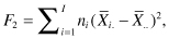
The comparison of more than two samples is an easy generalization of the method we used for comparing two samples. As in Chapter 4, we want a test statistic that takes more or less random values when there are no differences among the populations from which the samples are taken but tends to be large when there are differences. Suppose we have taken samples of sizes n1, n2, . . . nI from I distinct populations. Consider either of the statistics
that is, the weighted sum of the squared differences between the sample means and the grand means, where  is the mean of the ith sample and
  is the grand mean of all the observations, or
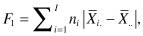
that is, the weighted sum of the absolute values of the differences between the sample means and the grand means.
Recall from Chapter 1 that the symbol Σ stands for sum of, so that

If the means of the I populations are approximately the same, then changing the labels on the various observations will not make any difference as to the expected value of F2 or F1, as all the sample means will still have more or less the same magnitude. On the other hand, if the values in the first population are much larger than the values in the other populations, then our test statistic can only get smaller if we start rearranging the observations among the samples.
Exercise 8.3: To demonstrate that this is true, at least for samples of size 2, cut pairs of sticks, the members of each pair having the length of one of the observations, and use the pairs to fence in areas.
Our permutation test consists of rejecting the hypothesis of no difference among the populations when the original value of F2 (or of F1 should we decide to use it as our test statistic) is larger than all but a small fraction, say 5%, of the possible values obtained by rearranging labels.
To program the analysis of more than two populations in R, we need to program an R function. We also make use of some new R syntax to sum only those data values that satisfy a certain condition, sum(data[condition]), as in the expression term=mean(data[start : end]) which computes the mean of the data items beginning with data[start] and ending with data[end].
 F1=function(size,data){
 #size is a vector containing the sample sizes
 #data is a vector containing all the data in the #same order as the sample sizes
 +  stat=0
 +  start=1
 + grandMean = mean(data)
+ for (i in 1:length(size)){
+   groupMean = mean(data[seq(from = start, length = size[i])])
+   stat = stat + abs(groupMean - grandMean)
+   start = start + size[i]
+   }
+  return(stat)
+ }
We use this function repeatedly in the following R program:
#One-way analysis of unordered data via a Monte #Carlo
size = c(4,6,5,4)
data = c(28,23,14.27, 33, 36,34, 29, 31, 34,
18,21,20,22,24,11,14,11,16)#Insert the definition of function F1 here
f1=F1(size,data)
#Number N of simulations determines precision of #p-value
N = 1600
cnt = 0
for (i in 1:N){ + pdata = sample (data) + f1p=F1(size,pdata) + #counting number of rearrangements for which F1 #greater than or equal to original + if (f1 <= f1p) cnt=cnt+1 + }
cnt/N
To test the program you’ve just created, generate 16 random values with the command
 data = rnorm(16, 2*rbinom(16, 1, .4))
The 16 values generated by this command come from a mixture of normal distributions N(0,1) and N(2,1). Set size = c(4,4,3,5). Now do the following exercises.
Exercise 8.4: Run your program to see if it will detect differences in these four samples despite their all being drawn from the same population.
Exercise 8.5: Modify your program by adding the following command after you’ve generated the data
 data = data + c(2,2,2,2, 0,0,0,0, 0,0,0, 0,0,0,0,0)
Now test for differences among the populations.
Exercise 8.6: We saw in the preceding exercise that if the expected value of the first population was much larger than the expected values of the other populations, we would have a high probability of detecting the differences. Would the same be true if the mean of the second population was much higher than that of the first? Why?
Exercise 8.7: Modify your program by adding the following command after you’ve generated the data
 data = data + c(1,1,1,1, 0,0,0,0, -1.2,-1.2,-1.2, 0 0,0,0,0)
Now test for differences among the populations.
*Exercise 8.8: Test your command of R programming; write a function to compute F2 and repeat the previous three exercises.
After you’ve created the function F1, you can save it to your hard disk with the R commands
 dir.create("C:/Rfuncs")  #if the directory does not yet exist
 save(F1, file="C:/Rfuncs/pak1.Rfuncs")
When you need to recall this function for use at a later time, just enter the command
 load("C:/Rfuncs/pak1.Rfuncs ")
We saw in the preceding exercises that we can detect differences among several populations if the expected value of one population is much larger than the others or if the mean of one of the populations is higher and the mean of a second population is lower than the grand mean.
Suppose we represent the expectations of the various populations as follows: EXi = μ + δi where μ (pronounced mu) is the grand mean of all the populations and δi (pronounced delta sub i) represents the deviation of the expected value of the ith population from this grand mean. The sum of these deviations Σδi = δ1 + δ2 + … δI = 0. We will sometimes represent the individual observations in the form Xij = μ + δi + zij, where zij is a random deviation with expected value 0 at each level of i. The permutation tests we describe in this section are applicable only if all the zij (termed the residuals) have the same distribution at each level of i.
One can show, though the mathematics is tedious, that the power of a test using the statistic F2 is an increasing function of Σδi2. The power of a test using the statistic F1 is an increasing function of Σ|δi|. The problem with these omnibus tests is that while they allow us to detect any of a large number of alternatives, they are not especially powerful for detecting a specific alternative. As we shall see in the next section, if we have some advance information that the alternative is an ordered dose response, for example, then we can develop a much more powerful statistical test specific to that alternative.
Exercise 8.9: Suppose a car manufacturer receives four sets of screws, each from a different supplier. Each set is a population. The mean of the first set is 4 mm, the second set 3.8 mm, the third set 4.1 mm and the fourth set 4.1 mm, also. What would the values of μ, δ1 , δ2, δ3, and δ4 be? What would be the value of Σ|δi|?
D. Frank et al. (1978)* studied the increase in chromosome abnormalities and micronuclei as the doses of various compounds known to cause mutations were increased. Their object was to develop an inexpensive but sensitive biochemical test for mutagenicity that would be able to detect even marginal effects. The results of their experiment are reproduced in Table 8.1.
Table 8.1 Micronucleii in Polychromatophilic Erythrocytes and Chromosome Alterations in the Bone Marrow of Mice Treated with CY
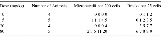
The best way to analyze these data is via the Pearson correlation applied not to the original doses but to their logarithms. To avoid problems with log(0), we add 1 to every dose before calculating its logarithm.
> logdose=log(c(rep(1,4),rep(6,5),rep(21,4),rep(81,5)))
> breaks= c(0, 1, 1, 2,   0, 1, 2, 3, 5,   3, 5, 7, 7,   6, 7, 8, 9, 9)
>  cor.test (logdose, breaks)
    Pearson's product-moment correlation
data: logdose and breaks
t = 6.8436, df = 16, p-value = 3.948e-06
alternative hypothesis: true correlation is not equal to 0
95 percent confidence interval:
0.6641900 0.9480747
sample estimates:     cor    0.863345
A word of caution: If we use as the weights some function of the dose other than g[dose] = log[dose+1], we might observe a different result. Our choice of a test statistic must always make practical as well as statistical sense. In this instance, the use of the logarithm was suggested by a pharmacologist.
Exercise 8.10: Using the data for micronuclei, see if you can detect a significant dose effect.
Exercise 8.11: Aflatoxin is a common and undesirable contaminant of peanut butter. Are there significant differences in aflatoxin levels among the following brands?
Snoopy = c(2.5, 7.3, 1.1, 2.7, 5.5, 4.3)
Quick = c(2.5, 1.8, 3.6, 4.2 , 1.2 ,0.7)
MrsGood = c(3.3, 1.5, 0.4, 2.8, 2.2 ,1.0)
(Hint: What is the null hypothesis? What alternative or alternatives are of interest?)
Exercise 8.12: Does the amount of potash in the soil affect the strength of fibers made of cotton grown in that soil? Consider the data in the following table:
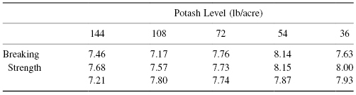
Exercise 8.13: Should you still perform this test if one or more of the observations in the previous table are missing?
Suppose that to cut costs on our weight-loss experiment, we have each participant weigh his or herself. Some individuals will make very precise measurements, perhaps repeating the procedure three or four times to make sure they’ve performed the measurement correctly. Others, will say “close enough,” and get the task done as quickly as possible. The problem with our present statistical methods is they treat each observation as if it were equally important. Ideally, we should give the least consideration to the most variable measurements and the greatest consideration to those that are least variable. The problem is that we seldom have any precise notion of what these variances are.
One possible solution is to put all results on a pass–fail or success–failure basis. This way, if the goal is to lose at least 7% of body weight, losses of 5 and 20% would offset each other, rather than a single 20% loss being treated as if it were equivalent to four losses of 5%. These pass-fail results would follow a binomial distribution and the appropriate method for testing binomial hypotheses could be applied.
The downside is the loss of information, but if our measurements are not equally precise, perhaps it is noise rather than useful information that we are discarding.
Here is a second example: An experimenter administered three drugs in random order to each of five recipients. He recorded their responses and now wishes to decide if there are significant differences among treatments. The problem is that the five subjects have quite different baselines. A partial solution would be to subtract an individual’s baseline value from all subsequent observations made on that individual. But who is to say that an individual with a high baseline value will respond in the same way as an individual with a low baseline reading?
An alternate solution would be to treat each individual’s readings as a block (see Section 6.2.3) and then combine the results. But then we run the risk that the results from an individual with unusually large responses might mask the responses of the others. Or, suppose the measurements actually had been made by five different experimenters using five different measuring devices in five different laboratories. Would it really be appropriate to combine them?
No, for sets of observations measured on different scales are not exchangeable. By converting the data to ranks, separately for each case, we are able to put all the observations on a common scale, and then combine the results.
When we replace observations by their ranks, we generally give the smallest value rank 1, the next smallest rank 2, and so forth. If there are N observations, the largest will have rank N. In creating Table 8.2b from Table 8.2a, we’ve made just such a transformation.
Table 8.2a Original Observations
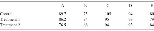
Table 8.2b Ranks
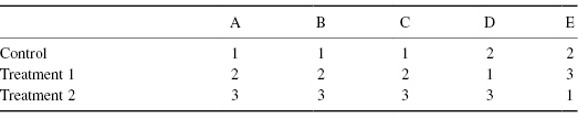
When three readings are made on each of five subjects, there are a total of (3!)5 = 7776 possible rearrangements of labels within blocks (subjects). For a test of the null hypothesis against any and all alternatives using F2 as our test statistic, as can be seen in Table 8.2b, only 2 × 5 = 10 of them, a handful of the total number of rearrangements, are as or more extreme than our original set of ranks.
Exercise 8.14: Suppose we discover that the measurement for Subject D for Treatment 1 was recorded incorrectly and should actually be 90. How would this affect the significance of the results depicted in Table 8.2?
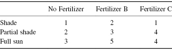
Exercise 8.15: Does fertilizer help improve crop yield when there is minimal sunlight? Here are the results of a recent experiment exactly as they were recorded. (Numbers in bushels.) No fertilizer: 5, 10, 8, 6, 9, 122. With fertilizer: 11, 18, 15, 14, 21, 14.
We have shown in two examples how one may test for the independence of continuous measurements using a correlation coefficient. But what if our observations are categorical involving race or gender or some other categorical attribute?
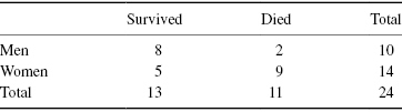
Suppose on examining the cancer registry in a hospital, we uncover the following data that we put in the form of a 2 × 2 contingency table (Table 8.3). At issue is whether cancer survival is a function of the patient’s sex.
Table 8.3 Cancer Survival as a Function of Sex
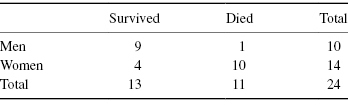
The 9 denotes the number of males who survived, the 1 denotes the number of males who died, and so forth. The four marginal totals or marginals are 10, 14, 13, and 11. The total number of men in the study is 10, while 14 denotes the total number of women, and so forth.
The marginals in this table are fixed because, indisputably, there are 11 dead bodies among the 24 persons in the study and 14 women. Suppose that before completing the table, we lost the subject IDs so that we could no longer identify which subject belonged in which category. Imagine you are given two sets of 24 labels. The first set has 14 labels with the word “woman” and 10 labels with the word “man.” The second set of labels has 11 labels with the word “dead” and 12 labels with the word “alive.” Under the null hypothesis that survival is independent of sex, you are allowed to distribute the two sets of labels to the subjects independently of one another. One label from each of the two sets per subject, please.
There are a total of  , 24 choose 10, ways you could hand out the gender labels “man” and “woman.”
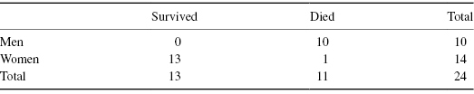
  of these assignments result in tables that are as extreme as our original table (i.e., in which 90% of the men survive), and
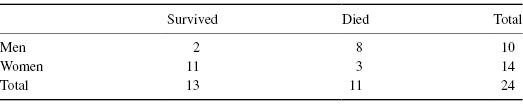
  in tables that are more extreme (100% of the men survive)—see Table 8.4a. In terms of the relative survival rates of the two sexes, Table 8.4a is more extreme than Table 8.3. Table 8.4b is less extreme.
Table 8.4a Cancer Survival, Same Row and Column Subtotals (marginals) as Table 8.3
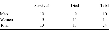
Table 8.4b Cancer Survival, Same Row and Column Subtotals (marginals) as Table 8.3
This is a very small fraction of the total number of possible tables with the same marginals, less than 1%. To show this explicitly, we will need the aid of two R functions that we program ourselves: one that will compute factorials and one that will compute combinations. The first of these takes advantage of our knowledge that n! = n(n − 1)! and uses a programming technique called recursion:
 fact=function(n){
+ if (n==1|n==0)1
+ else n*fact(n-1)
+ }
 fact=function(n){
+ if (n==1|n==0)1
+ else n*fact(n-1)
+ }
The preceding function assumes, without checking, that n is an integer. Let’s try again and provide some solution messages in case we forget when we try to use this function a year from now:
 fact=function(n){
+ if(n!=trunc(n))return(print("argument must be a whole number"))
+ if(n<0) return(print ("argument must be nonnegative integer"))
+ else if(n==0|n==1)return(1)
+ else return(n*fact(n-1))
}
 fact=function(n){
+ if(n!=trunc(n))return(print("argument must be a whole number"))
+ if(n<0) return(print ("argument must be nonnegative integer"))
+ else if(n==0|n==1)return(1)
+ else return(n*fact(n-1))
}
We then write  in the form
 comb = function (n,t) fact(n)/(fact(t)*fact(n-t))
We want to compute
 (10*comb(14,10) + comb(14,11))/comb(24,10)
[1] 0.0056142594
 (10*comb(14,10) + comb(14,11))/comb(24,10)
[1] 0.0056142594
From the result, 0.006, we conclude that a difference in survival rates of the two sexes at least as extreme as the difference we observed in our original table is very unlikely to have occurred by chance alone. We reject the hypothesis that the survival rates for the two sexes are the same and accept the alternative hypothesis that, in this instance at least, males are more likely to profit from treatment.
In our factorial program, we used the if() command along with some logical operators. These include
To combine conditions in a single if() use && meaning “and” or || meaning “or.”
Warning: If you write if(X=2)A instead of if(X==2)A, you will set X=2, and the statements A will always be executed.
If if(A)B is followed by else C, B will be executed if A is true and C will not be executed. If A is false, then C will be executed, but B will not be.
Exercise 8.16: Write an R program to test your understanding of the if() and else commands. Test your program using several different data sets.
The preceding test is known as Fisher’s exact test as it was first described by R.A. Fisher in 1935. Before we can write a program to perform this test, we need to consider the general case depicted in Table 8.5.
Table 8.5 Relationships among Entries in a Contingency Table

If the two attributes represented by the four categories are independent of one another, then each of the tables with the marginals n, m, and t is equally likely. If t is the smallest marginal, there are a total of  possible tables. If t — x is the value in the cell with the fewest observations, then

tables are as or more extreme than the one we observed.
Enter the actual cell frequencies
 data =c(f11, f12, f21, f22)
for example, data=c(9,1,4,10)
 data = array(data,dim=c(2,2)
 fisher.test(data)
Fisher’s Exact Test for Count Data
data:  data
p-value = 0.004526
alternative hypothesis: true odds ratio is not equal to 1
95 percent confidence interval for the odds ratio: 1.748845 1073.050540
sample estimates: odds ratio 19.18092
Exercise 8.17: a. Using the data in the following table, determine whether the new drug provides a statistically significant advantage over the old.
| Old Remedy | New Drug | |
| Improved | 6 | 10 |
| No improvement | 13 | 9 |
b. What must be true if this p-value is to be valid?
Exercise 8.18: What is the probability of observing Table 8.3 or a more extreme contingency table by chance alone?
Exercise 8.19: A physician has noticed that half his patients who suffer from sore throats get better within a week if they get plenty of bed rest. (At least they don’t call him back to complain they aren’t better.) He decides to do a more formal study and contacts each of 20 such patients during the first week after they’ve come to see him. What he learns surprises him. Twelve of his patients didn’t get much of any bed rest or if they did go to bed on a Monday, they were back at work on a Tuesday. Of these noncompliant patients, six had no symptoms by the end of the week. The remaining eight patients all managed to get at least three days bed rest (some by only going to work half-days) and of these, six also had no symptoms by the end of the week. Does bed rest really make a difference?
In the example of the cancer registry, we tested the hypothesis that survival rates do not depend on sex against the alternative that men diagnosed with cancer are likely to live longer than women similarly diagnosed. We rejected the null hypothesis because only a small fraction of the possible tables were as extreme as the one we observed initially. This is an example of a one-tailed test. But is it the correct test? Is this really the alternative hypothesis we would have proposed if we had not already seen the data? Wouldn’t we have been just as likely to reject the null hypothesis that men and women profit the same from treatment if we had observed a table of the following form?
Of course, we would! In determining the significance level in this example, we must perform a two-sided test and add together the total number of tables that lie in either of the two extremes or tails of the permutation distribution.
Unfortunately, it is not as obvious which tables should be included in the second tail. Is Table 8.6 as extreme as Table 8.3 in the sense that it favors an alternative more than the null hypothesis? One solution is simply to double the p-value we obtained for a one-tailed test. Alternately, we can define and use a test statistic as a basis of comparison. One commonly used measure is the Pearson χ2 (chi-square) statistic defined for the 2 × 2 contingency table after eliminating terms that are invariant under permutations as [x − tm/(m + n)]2. For Table 8.3, this statistic is 12.84; for Table 8.6, it is 29.34.
Table 8.6 Cancer Survival, Same Row and Column Subtotals (marginals) as Table 8.3
Exercise 8.20: Show that Table 8.7a is more extreme (in the sense of having a larger value of the chi-square statistic) than Table 8.3, but Table 8.7b is not.
Table 8.7a Cancer Survival, Same Row and Column Subtotals (marginals) as Table 8.3

Table 8.7b Cancer Survival, Same Row and Column Subtotals (marginals) as Table 8.3
Recall that in Table 3.1, we compared the observed spatial distribution of superclusters of galaxies with a possible theoretical distribution.
 observed = c(7178,2012,370,38,1,1)
 theoretical= c(7095,2144,324,32,2,0)
 data = c(observed, theoretical)
 dim(data)=c(6,2)
 fisher.test(data)
      Fisher's Exact Test for Count Data
      data:  data
      p-value = 0.05827
      alternative hypothesis: two.sided
It is possible to extend the approach described in the previous sections to tables with multiple categories, such as Table 8.8, Table 8.9, and Table 8.10.
Table 8.8 3 × 3 Contingency Table
Table 8.9 Oral Lesions in Three Regions of India
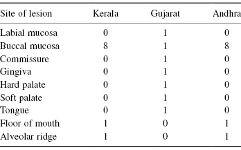
Table 8.10 Plant Survival Under Varying Conditions
As in the preceding sections, we need only to determine the total number of tables with the same marginals as well as the number of tables that are as or more extreme than the table at hand. Two problems arise. First, what do we mean by more extreme? In Table 8.8, would a row that held one more case of “Full Recovery” be more extreme than a table that held two more cases of “Partial Recovery?” At least a half-dozen different statistics, including the Pearson χ2 statistic, have been suggested for use with tables like of Table 8.9 in which neither category is ordered.
Exercise 8.21: In a two-by-two contingency table, once we fix the marginals, we are only free to modify a single entry. In a three-by-three table, how many different entries are we free to change without changing the marginals? Suppose the table has R rows and C columns, how many different entries are we free to change without changing the marginals?
The second problem that arises lies in the computations, which are not a simple generalization of the program for the 2 × 2 case. Fortunately, R is able to perform the Fisher–Freeman–Halton test. Consider the data in Table 8.9:
         Kerala = c(0,8,rep(0,5),1,1)
         Gujarat = c(rep(1,7),0,0)
         Andhra=Kerala
         data =c(Kerala,Gujarat,Andhra)
         nudata = array(data,dim=c(9,3))
         fisher.test(nudata)
    Fisher's Exact Test for Count Data
data:  nudata
p-value = 0.0101
alternative hypothesis: two.sided
Exercise 8.22: Apply the Fisher–Freeman–Halton test to the data of Table 8.10.
No competent physician would make a diagnosis on the basis of a single symptom. “Got a sore throat have you? Must be strep. Here take a pill.” To the contrary, she is likely to ask you to open your mouth and say, “ah,” take your temperature, listen to your chest and heartbeat, and perhaps take a throat culture. Similarly, a multivariate approach is far more likely to reveal differences brought about by treatment or environment than focusing on changes in a single endpoint.
Will a new drug help mitigate the effects of senility? To answer this question, we might compare treated and control patients on the basis of their scores on three quizzes: current events, arithmetic, and picture completion.
Will pretreatment of seeds increase the percentage of germination, shorten the time to harvest, and increase the yield?
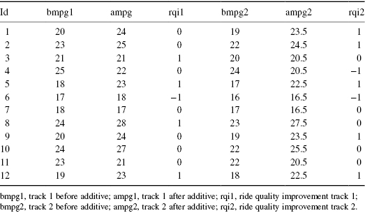
Will a new fuel additive improves gas mileage and ride quality in both stop-and-go and highway situations?
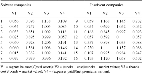
In trying to predict whether a given insurance firm can avoid bankruptcy, should we measure the values and ratios of agents balances, total assets, stocks less cost, stocks less market value, expenses paid, and net premiums written?
In Section 8.5.2, we will learn how to combine the p-values obtained from separate but dependent single-variable (univariate) tests into an overall multivariate p-value.
To take advantage of multivariate statistical procedures, we need to maintain all the observations on a single experimental unit as a single indivisible vector. If we are to do a permutation test, labels must be applied to and exchanged among these vectors and not among the individual observations. For example, if we are studying the effects of pretreatment on seeds, the data for each plot (the number of seeds that germinated, the time to the initial harvest, and the ultimate yield) must be treated as a single indivisible unit.
Data for the different variables may have been entered in separate vectors
 germ = c(11,9,8,4)
 time = c(5, 4.5, 6, 8)
Or, the observations on each experimental unit may have been entered separately.
 one = c(11,5)
 two = c (9,4.5)
 thr = c(8,6)
 four = c(4,8)
In the first case, we put the data in matrix form as follows
 temp = c(germ,time)
 data = matrix(temp,2,4, byrow=T)
 data
  [,1] [,2] [,3] [,4]
[1,]   11  9.0    8    4
[2,]    5  4.5    6    8
If the observations on each experimental unit have been entered separately, we would create a matrix this way;
 temp = c(one,two,thr, four)
 data = matrix (temp, 2,4)
 data
  [,1] [,2] [,3] [,4]
[1,]   11  9.0    8    4
[2,]    5  4.5    6    8
We can rank all the observations on a variable-by-variable basis with the commands
 R1 = rank(data[1,])
 R2 = rank(data[2,])
 rdata = matrix(c(R1,R2),2,4,byrow=T)
Here is a useful R function for generating random rearrangements of multivariate data:
 rearrange =function (data){
n=length(data[1, ])
m= length (data[ ,1])
vect = c(1:n)
rvect = sample (vect)
new = data
for (j in 1:n){
ind = rvect [j]
for (k in 1:m) new[k,j]= data [k,ind]
}
return(new)
}
 rearrange =function (data){
    n=length(data[1, ])
    m= length (data[ ,1])
    vect = c(1:n)
    rvect = sample (vect)
    new = data
    for (j in 1:n){
         ind = rvect [j]
         for (k in 1:m)  new[k,j]= data [k,ind]
         }
  return(new)
}In the univariate (single-variable) case, Student’s t and R’s t.test serve for the comparison of the means of two populations and permutation tests are seldom necessary except for very small samples. Unlike Student’s t, Hotelling’s T2, the multivariate equivalent of Student’s t, is highly sensitive to departures from normality, and a distribution-free permutation approach to determining a p-value is recommended. To perform a permutation test with multivariate observations, we treat each vector of observations on an individual subject as a single indivisible entity. When we rearrange the treatment labels, we relabel on a subject-by-subject basis so that all observations on a single subject receive the same new treatment label.
Proceed in three steps:
#This function for computing Hotelling's T2 is due to Nick Horton
hotelling = function(y1, y2) {
  #check the appropriate dimension
  k = ncol(y1)
  k2 = ncol(y2)
  if (k2!=k)
    stop("input matrices must have the same number of columns: y1 has ",
    k, " while y2 has ", k2)

  #calculate sample size and observed means
  n1 = nrow(y1)
  n2 = nrow(y2)
  ybar1 = apply(y1, 2, mean); ybar2 = apply(y2, 2, mean)
  diffbar = ybar1-ybar2

  #calculate the variance of the difference in means
  v = ((n1-1)*var(y1) + (n2-1)*var(y2))/(n1+n2-2)

  #calculate the test statistic and associated #quantities
  #%x% multiplies two matrices
  t2 = n1*n2*diffbar%*%solve(v)%*%diffbar/(n1+n2)
  f = (n1+n2-k-1)*t2/((n1+n2-2)*k)
  pvalue = 1-pf(f, k, n1+n2-k-1)

  #return the list of results
  return(list(pvalue=pvalue, f=f, t2=t2, diff=diffbar))
}
#Compute the exact p-value
photell= function (samp1,samp2,fir,last,MC){
#fir=first of consecutive variables to be included in #the analysis
#last=last of consecutive variables to be included in #the analysis
#compute lengths of samples
d1=dim(samp1)[1]
d2=dim(samp2)[1]
d=d1+d2
samp=c(samp1,samp2)
#create dataframe to hold rearranged data
nsamp=samp
#compute test statistic for data
res=hotelling(samp[1:d1, fir:last],samp[(1+d1):d,fir:last])
stat0=as.numeric(res[[3]])
#run Monte Carlo simulation of p-value
cnt=1
for (j in 1:MC){
     nu=sample(lgth)
     for (k in 1:d)nsamp[nu[k],]=samp[k,]
     res=hotelling(nsamp[1:d1, fir:lst],nsamp[(1+d1):d, fir:last])
     if (as.numeric(res[[3]])>=stat0)cnt=cnt+1
     }
return (cnt)
}
print(c("pvalue=",cnt/MC), quote=FALSE)
Let Data denote the original N × M matrix of multivariate observations. N, the number of rows in the matrix, corresponds to the number of experimental units. M, the number of columns in this matrix, corresponds to the number of different variables.
Our first task is to replace the matrix by a row vector T0 of M univariate statistics. That is, calculating a column at a time, we replace that column with a single value—a t-statistic, a mean, or some other value.
To fix ideas, suppose we wish to compare two lots of fireworks, and have taken a sample from each. For each firework, we have recorded whether or not it exploded, how long it burned, and some measure of its brightness. The first column of the Data matrix consists of a series of ones corresponding to whether or not the firework for that row exploded. Such observations are best evaluated by the methods of Section 8.4, so we replace the column by a single number, that of the value of the Pearson chi-square statistic.
The times that are recorded in the second column have approximately an exponential distribution (see Section 4.4). So unless the observation is missing (as it would be if the firework did not explode), we take its logarithm, and replace the column by the mean of the observations in the first sample.
The brightness values in the third column have approximately a normal distribution, so we replace this column by the corresponding value of the t-statistic.
Our second task is to rearrange the observations in DATA between the two samples, using the methods of the previous section so as to be sure to keep all the observations on a given experimental unit together. Again, we compute a row vector of univariate statistics T. We repeat this resampling process K times. If there really isn’t any difference between the two lots of fireworks, then each of the vectors Tk obtained after rearranging the data as well as the original vector T0 are equally likely.
We would like to combine these values but have the same problem we encountered and resolved in Section 8.3: the p-values have all been measured on different scales. The solution as it was in Section 8.3 is to replace the K + 1 different values of each univariate test statistic by their ranks. We rank the K + 1 values of the χ2 statistic separately from the K + 1 values of the t-statistic, and so forth, so that we have m sets of ranks ranging from 1 to K + 1.
The ranks should be related to the extent to which the statistic favors the alternative. For example, if large values of the t-statistic are to be expected when the null hypothesis is false, then the largest value of this statistic should receive rank K + 1.
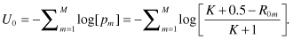
Our third task is to combine the ranks of the M individual univariate tests using Fisher’s omnibus statistic
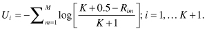
Our fourth and final task is to determine the p-value associated with this statistic. We require three sets of computations. To simplify writing them down, we will make repeated use of an indicator function I. I[y] = 1 if its argument y is true, I[y] = 0 otherwise. For example, I[T>3] is 1 if T > 3 and is 0 otherwise.


To perform the Pesarin–Fisher omnibus multivariate test, you will need to write a program in R. The program is a long one and it is essential that you proceed in a systematic fashion. Here are some guidelines.
Anticipate and program for exceptions. For example:
if (n<0 || k<0 || (n-trunc(n))!=0 || (k-trunc(k))!=0) stop("n and k must be positive integers")else fact(n)/(fact(k)*fact(n-k))
Testing and debugging a program also requires that you proceed in a systematic fashion:
Once you are sure your program works correctly, you can remove these redundant commands.
Exercise 8.23: You are studying a new tranquilizer that you hope will minimize the effects of stress. The peak effects of stress manifest themselves between 5 and 10 minutes after the stressful incident, depending on the individual. To be on the safe side, you’ve made observations at both the 5- and 10-minute marks.
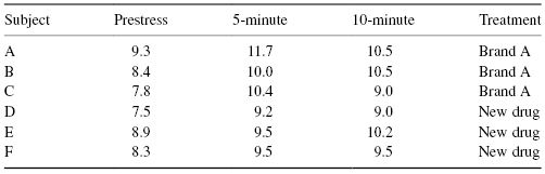
How would you correct for the prestress readings? Is this a univariate or a multivariate problem? List possible univariate and multivariate test statistics. Perform the permutation tests and compare the results.
Exercise 8.24: To help understand the sources of insolvency, J. S. Trieschman and G. E. Pinches (1973)* compared the financial ratios of solvent and financially distressed insurance firms. A partial listing of their findings is included in the following table. Are the differences statistically significant? Be sure to state the specific hypotheses and alternative hypotheses you are testing. Will you use Student’s t as your univariate test statistic each time? Or the difference in mean values? Or simply the sum of the observations in the first sample?
Exercise 8.25: You wish to test whether a new fuel additive improves gas mileage and ride quality in both stop-and-go and highway situations. Taking 12 vehicles, you run them first on a highway-style track and record the gas mileage and driver’s comments. You then repeat on a stop-and-go track. You empty the fuel tanks and refill, this time including the additive, and again run the vehicles on the two tracks.
The following data were supplied in part by the Stata Corporation. Use Pesarin’s combination method to test whether the additive affects either gas mileage or ride quality.
Exercise 8.26: The following data are based on samples taken from swimming areas off the coast of Milazzo (Italy) from April through September 1998. Included in this data set are levels of total coliform, fecal coliform, streptococci, oxygen, and temperature.
Month = c(4, 5, 6, 7, 8, 9, 4, 5, 6, 7, 8, 9, 4, 5, 6, 7, 8, 9, 4, 5, 6, 7, 8, 9, 4, 5, 6, 7, 8, 9, 4, 5, 6, 7, 8, 9, 4, 5, 6, 7, 8, 9, 4, 5, 6, 7, 8, 9, 4, 5, 6, 7, 8, 9, 4, 5, 6, 7, 8, 9, 4, 5, 6, 7, 8, 9, 4, 5, 6, 7, 8, 9, 4, 5, 6, 7, 8, 9, 4, 5, 6, 7, 8, 9)
Temp = c(14, 17, 24, 21, 22, 20, 14, 17, 24, 21, 23, 22, 14, 17, 25, 21, 21, 22, 14, 17, 25, 21, 25, 20, 14, 17, 25, 21, 21, 19, 14, 17, 25, 21, 25, 19, 14, 16, 25, 21, 25, 19, 15, 19, 18, 21, 25, 19, 15, 19, 18, 20, 22, 17, 15, 19, 18, 20, 23, 18, 15, 17, 18, 20, 25, 17, 15, 17, 18, 20, 25, 19, 15, 17, 19, 20, 25, 18, 15, 18, 19, 21, 24, 19)
TotColi = c(30, 22, 16, 18, 32, 40, 50, 34, 32, 32, 34, 18, 16, 19, 65, 54, 32, 59, 45, 27, 88, 32, 78, 45, 68, 14, 54, 22, 25, 32, 22, 17, 87, 17, 46, 23, 10, 19, 38, 22, 12, 26, 8, 8, 11, 19, 45, 78, 6, 9, 87, 6, 23, 28, 0, 0, 43, 8, 23, 19, 0, 5, 28, 19, 14, 32, 12, 17, 33, 21, 18, 5, 22, 13, 19, 27, 30, 28, 16, 6, 21, 27, 58, 45)
FecColi = c(16, 8, 8, 11, 11, 21, 34, 11, 11, 7, 11, 6, 8, 6, 35, 18, 18, 21, 13, 9, 32, 11, 29, 11, 28, 7, 12, 7, 12, 9, 10, 3, 43, 5, 12, 14, 4, 9, 8, 10, 4, 12, 0, 4, 7, 5, 12, 26, 0, 3, 32, 0, 8, 12, 0, 0, 21, 0, 7, 8, 0, 0, 17, 4, 0, 14, 0, 0, 11, 7, 6, 0, 8, 0, 6, 4, 5, 10, 14, 3, 8, 12, 11, 27)
Strep = c(8, 4, 3, 5, 6, 9, 18, 7, 6, 3, 5, 2, 6, 0, 11, 2, 12, 7, 9, 3, 8, 6, 9, 4, 8, 2, 7, 3, 5, 3, 4, 0, 16, 0, 6, 5, 0, 0, 2, 4, 0, 4, 0, 0, 3, 0, 5, 14, 0, 0, 11, 0, 2, 4, 0, 0, 3, 0, 2, 2, 0, 0, 7, 2, 0, 5, 0, 0, 7, 4, 3, 0, 2, 0, 2, 2, 3, 5, 8, 1, 2, 4, 5, 7)
O2 = c(95.64, 102.09, 104.76, 106.98, 102.6, 109.15, 96.12, 111.98, 100.67, 103.87, 107.57, 106.55, 89.21, 100.65, 100.54, 102.98, 98, 106.86, 98.17, 100.98, 99.78, 100.87, 97.25, 97.78, 99.24, 104.32, 101.21, 102.73, 99.17, 104.88, 97.13, 102.43, 99.87, 100.89, 99.43, 99.5, 99.07, 105.32, 102.89, 102.67, 106.04, 106.67, 98.14, 100.65, 103.98, 100.34, 98.27, 105.69, 96.22, 102.87, 103.98, 102.76, 107.54, 104.13, 98.74, 101.12, 104.98, 101.43, 106.42, 107.99, 95.89, 104.87, 104.98, 100.89, 109.39, 98.17, 99.14, 103.87, 103.87, 102.89, 108.78, 107.73, 97.34, 105.32, 101.87, 100.78, 98.21, 97.66, 96.22, 22, 99.78, 101.54, 100.53, 109.86)
In this chapter, you learned to analyze a variety of different types of experimental data. You learned to convert your data to logarithms when changes would be measured in percentages or when analyzing data from dividing populations. You learned to convert your data to ranks when observations were measured on different scales or when you wanted to minimize the importance of extreme observations.
You learned to specify in advance of examining your data whether your alternative hypotheses of interest were one-sided or two-sided, ordered or unordered.
You learned how to compare binomial populations and to analyze 2 × 2 contingency tables. You learned how to combine the results of multiple endpoints via Hotelling’s T2 and the Pesarin–Fisher omnibus multivariate test.
You were introduced to the built-in R math functions log, exp, rank, abs, and trunc , used R functions cor.test and fisher.test and created several new R functions of your own with the aid of if … else commands and return(list()). You learned how to store data in matrix form using the R functions array, dim, and matrix, multiply matricies using %*%, and extract the marginal of matricies using the apply function. You learned how to print results along with techniques for the systematic development and testing of lengthy programs.
Exercise 8.27: Write definitions for all italicized words in this chapter.
Exercise 8.28: Many surveys employ a nine-point Likert scale to measure respondent’s attitudes where a value of “1” means the respondent definitely disagrees with a statement and a value of “9” means they definitely agree. Suppose you have collected the views of Republicans, Democrats, and Independents in just such a form. How would you analyze the results?
Notes
* Evaluating drug-induced chromosome alterations, Mutation Res. 1978; 56: 311–317.
* A multivariate model for predicting financially distressed P-L insurers, J. Risk Insurance. 1973; 40: 327–338.