 Time = c(0.5,1,1.5,2, 2.5, 3)
 S = 60*Time
 plot(S, xlab="Time")
Chapter 9
Developing Models
A recent help wanted ad touted openings with a sportsbook; they were looking for statisticians who could help them develop real-time software for forecasting the outcomes of cricket matches. In this chapter, you will learn valuable techniques with which to develop forecasts and classification schemes. These techniques have been used to forecast parts s4ales by the Honda Motors Company and epidemics at naval training centers, to develop criteria for retention of marine recruits, optimal tariffs for Federal Express, and multitiered pricing plans for Delta Airlines. And these are just examples in which I’ve been personally involved!
A model in statistics is simply a way of expressing a quantitative relationship between one variable, usually referred to as the dependent variable, and one or more other variables, often referred to as the predictors. We began our text with a reference to Boyle’s law for the behavior of perfect gases, V = KT/P. In this version of Boyle’s law, V (the volume of the gas) is the dependent variable; T (the temperature of the gas) and P (the pressure exerted on and by the gas) are the predictors; and K (known as Boyle’s constant) is the coefficient of the ratio T/P.
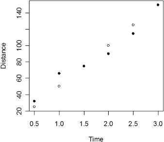
An even more familiar relationship is that between the distance S traveled in t hours and the velocity V of the vehicle in which we are traveling: S = Vt. Here, S is the dependent variable, and V and t are predictors. If we travel at a velocity of 60 mph for 3 hours, we can plot the distance we travel over time, using the following R code:
I attempted to drive at 60 mph on a nearby highway past where a truck had recently overturned with the following results:
 SReal = c(32,66,75,90,115,150)
 plot(Time,S, ylab="Distance")
 points(Time,SReal,pch=19)
As you can see, the reality was quite different from the projected result. My average velocity over the 3-hour period was equal to distance traveled divided by time or 150/3 = 50 mph. That is, Si = 50*Timei + zi, where the {zi} are random deviations from the expected distance.
Let’s compare the new model with the reality:
 S = 50*Time
 SReal = c(32,66,75,90,115,150)
 plot(Time,S, ylab="Distance")
 points(Time,SReal,pch=19)
Our new model, depicted in Figure 9.1, is a much better fit, agreed?
Figure 9.1 Distance expected at 50 mph versus distance observed.
We develop models for at least three different purposes. First, as the terms “predictors” suggests, models can be used for prediction. A manufacturer of automobile parts will want to predict part sales several months in advance to ensure its dealers have the necessary parts on hand. Too few parts in stock will reduce profits; too many may necessitate interim borrowing. So entire departments are hard at work trying to come up with the needed formula.
At one time, I was part of just such a study team working with Honda Motors. We soon realized that the primary predictor of part sales was the weather. Snow, sleet, and freezing rain sent sales skyrocketing. Unfortunately, predicting the weather is as or more difficult than predicting part sales.
Second, models can be used to develop additional insight into cause and effect relationships. At one time, it was assumed that the growth of the welfare case load L was a simple function of time t, so that L = ct, where the growth rate c was a function population size. Throughout the 1960s, in state after state, the constant c constantly had to be adjusted upward if this model were to fit the data. An alternative and better fitting model proved to be L = ct + dt2, an equation often used in modeling the growth of an epidemic. As it proved, the basis for the new second-order model was the same as it was for an epidemic: Welfare recipients were spreading the news of welfare availability to others who had not yet taken advantage of the program much as diseased individuals might spread an infection.
Boyle’s law seems to fit the data in the sense that if we measure both the pressure and volume of gases at various temperatures, we find that a plot of pressure times volume versus temperature yields a straight line. Or if we fix the volume, say by confining all the gas in a chamber of fixed size with a piston on top to keep the gas from escaping, a plot of the pressure exerted on the piston against the temperature of the gas yields a straight line.
Observations such as these both suggested and confirmed what is known today as kinetic molecular theory.
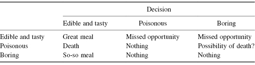
A third use for models is in classification. At first glance, the problem of classification might seem quite similar to that of prediction. Instead of predicting that Y would be 5 or 6 or even 6.5, we need only predict that Y will be greater or less than 6, for example. A better example might be assigning a mushroom as one of the following classifications: (1) edible and tasty, (2) poisonous, and (3) boring. The loss functions for prediction and classification are quite different. The loss connected with predicting yp when the observed value is yo is usually a monotone increasing function of the difference between the two. By contrast, the loss function connected with a classification problem has jumps, as in Table 9.1.
Table 9.1 Classification Loss Matrix for Mushroom Example
Not surprisingly, different modeling methods have developed to meet the different purposes. In the balance of the chapter, we shall consider three primary modeling methods: decision trees, which may be used both for classification and prediction, linear regression, whose objective is to predict the expected value of a given dependent variable, and quantile regression, whose objective is to predict one or more quantiles of the dependent variable’s distribution.
The modeling techniques that you learn in this chapter may seem impressive—they require extensive calculations that only a computer can do—so that I feel it necessary to issue three warnings.
You may have heard that a black cat crossing your path will bring bad luck. Don’t step in front of a moving vehicle to avoid that black cat unless you have some causal basis for believing that black cats can affect your luck. (And why not white cats or tortoise shell?) I avoid cats myself because cats lick themselves and shed their fur; when I breathe cat hairs, the traces of saliva on the cat fur trigger an allergic reaction that results in the blood vessels in my nose dilating. Now, that is a causal connection.
If you’re a mycologist, a botanist, a herpetologist or simply a nature lover you may already have made use of some sort of a key. For example,
The R rpart() procedure attempts to construct a similar classification scheme from the data you provide. You’ll need to install a new package of R functions in order to do the necessary calculations. The easiest way to do this is get connected to the Internet and then type
 install.packages("rpart")
The installation which includes downloading, unzipping, and integrating the new routines is then done automatically. Installation needs to be done once and once only. But each time, you’ll need to load the decision-tree building functions into computer memory before you can us them by typing
 library(rpart)
In order to optimize an advertising campaign for a new model of automobile by directing the campaign toward the best potential customers, a study of consumers’ attitudes, interests, and opinions was commissioned. The questionnaire consisted of a number of statements covering a variety of dimensions, including consumers’ attitudes towards risk, foreign-made products, product styling, spending habits, emissions, pollution, self-image, and family. The final question concerned the potential customer’s attitude toward purchasing the product itself. All responses were tabulated on a nine-point Likert scale. The data may be accessed at http://statcourse.com/Data/ConsumerSurvey.htm.
Figure 9.2 is an example of a decisions tree we constructed using the data from the consumer survey and the R commands
 catt.tr=rpart(Purchase ∼Fashion + Ozone + Gamble)
 plot(catt.tr, uniform=TRUE, compress=TRUE);
text(catt.tr, use.n=TRUE)
Figure 9.2 Labeled regression tree for predicting purchase attitude.
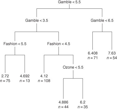
Note that some of the decisions, that is, the branch points in the tree shown in the figure, seem to be made on the basis of a single predictor—Gamble; others utilized the values of two predictors—Gamble and Fashion; and still others utilized the values of Gamble, Fashion, and Ozone, the equivalent of three separate linear regression models.
Exercise 9.1: Show that the R function rpart() only makes use of variables it considers important by constructing a regression tree based on the model

Exercise 9.2: Apply the computer-aided regression tree (CART) method to the Milazzo data of the previous chapter in Exercise 8.24 to develop a prediction scheme for coliform levels in bathing water based on the month, oxygen level, and temperature.
The output from our example and from Exercises 9.1 and 9.2 are regression trees, that is, at the end of each terminal node is a numerical value. While this might be satisfactory in an analysis of our Milazzo coliform data, it is misleading in the case of our consumer survey, where our objective is to pinpoint the most likely sales prospects.
Suppose instead that we begin by grouping our customer attitudes into categories. Purchase attitudes of 1, 2, or 3 indicate low interest, 4, 5, and 6 indicate medium interest, 7, 8, and 9 indicate high interest. To convert them using R, we enter
 Pur.cat = cut(Purchase,breaks=c(0,3,6,9),labels=c("lo", "med", "hi"))
Now, we can construct the classification tree depicted in Figure 9.3.
 catt.tr=rpart(Pur.cat∼Fashion + Ozone + Gamble)
 plot(catt.tr, uniform=TRUE, compress=TRUE);
text(catt.tr, use.n=TRUE)
Figure 9.3 Labeled classification tree for predicting prospect attitude.
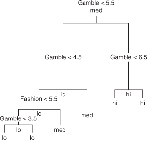
Many of the branches of this tree appear redundant. If we have already classified a prospect, there is no point in additional questions. We can remove the excess branches and create a display similar to Figure 9.4 with the following code:
 tmp=prune(catt.tr, cp=0.02)
 plot(tmp); text(tmp)
Figure 9.4 Pruned classification tree for predicting prospect attitude.

These classifications are actually quite tentative; typing the command
 print(tmp)
will display the nodes in this tree along with the proportions of correct and incorrect assignments.
n = 400
node), split, n, loss, yval, (yprob)
    * denotes terminal node
1) root 400 264 med (0.3375000 0.3400000 0.3225000)
  2) Gamble< 5.5 275 148 lo (0.4618182 0.3600000 0.1781818)
    4) Gamble< 4.5 192  83 lo (0.5677083 0.2708333 0.1614583)
      8) Fashion< 5.5 160  57 lo (0.6437500 0.2375000 0.1187500) *
      9) Fashion>=5.5 32  18 med (0.1875000 0.4375000 0.3750000) *
    5) Gamble>=4.5 83  36 med (0.2168675 0.5662651 0.2168675) *
  3) Gamble>=5.5 125  45 hi (0.0640000 0.2960000 0.6400000) *
The three fractional values within parentheses refer to the proportions in the data set that were assigned to the “low,” “med,” and “hi” categories, respectively. For example, in the case when Gamble > 5.5, 64% are assigned correctly by the classification scheme, while just over 6% who are actually poor prospects (with scores of 3 or less) are assigned in error to the high category.
Exercise 9.3: Goodness of fit does not guarantee predictive accuracy. To see this for yourself, divide the consumer survey data in half. Use the first part for deriving the tree, and the second half to validate the trees use for prediction.
Classification and regression tree builders like rpart() make binary splits based on either yes/no (Sex = Male?) or less than/greater than (Fashion < 5.5) criteria. The tree is built a level at a time beginning at the root. At each level, the computationally intensive algorithm used by rpart() examines each of the possible predictors and chooses the predictor and the split value (if it is continuous) that best separates the data into more homogenous subsets.
 This method is illustrated in Figures 9.5a,b and 9.6 using the iris data set at http://statcourse.com/research/Iris.csv. The objective in this instance is to assign an iris to one of three species based on the length and width of its petals and its sepals.
Figure 9.5 Subdividing iris into species by a single variable: (a) petal length, (b) sepal length.
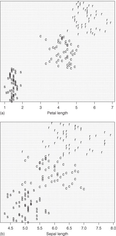
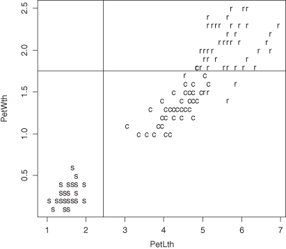
Figure 9.6 Classifying iris into species by petal length and petal width.
The best fitting decision tree is
 rpart(Class∼SepLth + PetLth + SepWth + PetWth)
node), split, n, loss, yval, (yprob)
* denotes terminal node
1) root 150 100 setosa (0.33333333 0.33333333 0.33333333)
2) PetLth< 2.45 50 0 setosa (1.00000000 0.00000000 0.00000000) *
3) PetLth>=2.45 100 50 versicolor (0.00000000 0.50000000 0.50000000)
6) PetWth< 1.75 54 5 versicolor (0.00000000 0.90740741 0.09259259) *
7) PetWth>=1.75 46 1 virginica (0.00000000 0.02173913 0.97826087) *
 rpart(Class∼SepLth + PetLth + SepWth + PetWth)
node), split, n, loss, yval, (yprob)
   * denotes terminal node
1) root 150 100 setosa (0.33333333 0.33333333 0.33333333)
  2) PetLth< 2.45 50   0 setosa (1.00000000 0.00000000 0.00000000) *
  3) PetLth>=2.45 100  50 versicolor (0.00000000 0.50000000 0.50000000)
    6) PetWth< 1.75 54   5 versicolor (0.00000000 0.90740741 0.09259259) *
    7) PetWth>=1.75 46   1 virginica (0.00000000 0.02173913 0.97826087) *
in which sepal length and width play no part.
One can and should incorporate one’s knowledge of prior probabilities and relative costs into models built with a classification and regression tree. In particular, one can account for all of the following:
When decision trees are used for the purpose of analyzing biomedical images—sonograms, X-rays, EEGs, and PET scans, all three of these factors must be taken into consideration.
Although equal numbers of the three species of Iris were to be found in the sample studied by Anderson, it is highly unlikely that you would find such a distribution in an area near where you live. Specifying that the setosa are the most plentiful yields a quite different decision tree. In the following R code, we specify that the setosa occur 60% of the time:
 rpart(Class∼SepLth + PetLth + SepWth + PetWth, parms=list(prior=c(.20,.20,.60)))
1) root 150 60.0 virginica (0.20000000 0.20000000 0.60000000)
2) PetLth< 4.75 95 28.2 setosa (0.51546392 0.45360825 0.03092784)
4) PetLth< 2.45 50 0.0 setosa (1.00000000 0.00000000 0.00000000) *
5) PetLth>=2.45 45 1.8 versicolor (0.00000000 0.93617021 0.06382979) *
3) PetLth>=4.75 55 3.6 virginica (0.00000000 0.03921569 0.96078431) *
 rpart(Class∼SepLth + PetLth + SepWth + PetWth, parms=list(prior=c(.20,.20,.60)))
  1) root 150 60.0 virginica (0.20000000 0.20000000 0.60000000)
    2) PetLth< 4.75 95 28.2 setosa (0.51546392 0.45360825 0.03092784)
      4) PetLth< 2.45 50  0.0 setosa (1.00000000 0.00000000 0.00000000) *
      5) PetLth>=2.45 45  1.8 versicolor (0.00000000 0.93617021 0.06382979) *
3) PetLth>=4.75 55 3.6 virginica (0.00000000 0.03921569 0.96078431) *Suppose instead of three species of Iris, we had data on three species of mushroom: the Amanita calyptroderma (edible and choice), Amanita citrine (probably edible), and the Aminita verna (more commonly known as the Destroying Angel). Table 9.1 tells us that the losses from misclassification vary from a missed opportunity at a great meal to death. We begin by assigning numeric values to the relative losses and storing these in a matrix with zeros along its diagonal:
 M = c(0,1, 2,100,0, 50,1,2,0)
 dim(M) = c(3,3
 rpart(species∼CapLth + Volvath + Capwth + Volvasiz,
  parms=list(loss=M)))
1) root 150 150 A.verna (0.3333333 0.3333333 0.3333333)
   2) Volvasiz< 0.8 50   0 A.citrina (1.0000000 0.0000000 0.0000000) *
   3) Volvasiz>=0.8 100 100 A.verna (0.0000000 0.5000000 0.5000000)
      6) Volvasiz< 1.85 66  32 A.verna (0.0000000 0.7575758 0.2424242)
     12) Volvath< 5.3 58  16 A.verna (0.0000000 0.8620690 0.1379310) *
     13) Volvath>=5.3 8   0 A.calyptroderma (0.0000000 0.0000000 1.0000000) *
      7) Volvasiz>=1.85 34   0 A.calyptroderma (0.0000000 0.0000000 1.0000000) *
Note that the only assignments to edible species (the group of three values in parentheses at the end of each line) made in this decision tree are those which were unambiguous in the original sample. All instances, which by virtue of their measurements, might be confused with the extremely poisonous Amanita verna are classified as Amanita verna. A wise decision indeed!
Exercise 9.4: Develop a decision tree for classifying breast tumors as benign or malignant using the data at http://archive.ics.uci.edu/ml/datasets/Breast+Cancer+Wisconsin+(Diagnostic).
Account for the relative losses of misdiagnosis.
Regression combines two ideas with which we gained familiarity in previous chapters:
Here is an example: Anyone familiar with the restaurant business (or indeed, with any number of businesses which provide direct service to the public, including the Post Office) knows that the volume of business is a function of the day of the week. Using an additive model, we can represent business volume via the formula
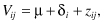
where Vij is the volume of business on the ith day of the jth week, μ is the average volume, δi is the deviation from the average volume observed on the ith day of the week, i = 1, . . . , 7, and the zij are independent, identically distributed random fluctuations.
Many physiological processes such as body temperature have a circadian rhythm, rising and falling each 24 hours. We could represent temperature by the formula
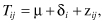
where i (in minutes) takes values from 1 to 24*60, but this would force us to keep track of 1441 different parameters. Besides, we can get almost as good a fit to the data using a formula with just two parameters, μ and β as in Equation 9.1:
If you are not familiar with the cos() trigonometric function, you can use R to gain familiarity as follows:
 hour = c(0:24)
 P = cos(2*pi*(hour + 6)/24)
 plot(P)
Note how the cos() function first falls then rises, undergoing a complete cycle in a 24-hour period.
Why use a formula as complicated as Equation 9.1? Because now we have only two parameters we need to estimate, μ and β. For predicting body temperature μ = 98.6 and β = 0.4 might be reasonable choices, though, of course, the values of these parameters will vary from individual to individual. For the author of this text, his mean body temperature is μ = 97.6°F.
Exercise 9.5: If E(Y) = 3X + 2, can X and Y be independent?
Exercise 9.6: According to the inside of the cap on a bottle of Snaple’s Mango Madness, “the number of times a cricket chirps in 15 seconds plus 37 will give you the current air temperature.” How many times would you expect to hear a cricket chirp in 15 seconds when the temperature is 39°? 124°?
Exercise 9.7: If we constantly observe large values of one variable, call it Y, whenever we observe large values of another variable, call it X, does this mean X is part of the mechanism responsible for increases in the value of Y? If not, what are the other possibilities? To illustrate the several possibilities, give at least three real-world examples in which this statement would be false. (You’ll do better at this exercise if you work on it with one or two others.)
Equation 9.1 is an example of linear regression. The general form of linear regression is
(9.2) 
where Y is known as the dependent or response variable, X is known as the independent variable or predictor, f[X] is a function of known form, μ and β are unknown parameters, and Z is a random variable whose expected value is zero. If it weren’t for this last random component Z, then if we knew the parameters μ and β, we could plot the values of the dependent variable Y and the function f[X] as a straight line on a graph. Hence the name, linear regression.
For the past year, the price of homes in my neighbor could be represented as a straight line on a graph relating house prices to time. P = μ + βt, where μ was the price of the house on the first of the year and t is the day of the year. Of course, as far as the price of any individual house was concerned, there was a lot of fluctuation around this line depending on how good a salesman the realtor was and how desperate the owner was to sell.
If the price of my house ever reaches $700 K, I might just sell and move to Australia. Of course, a straight line might not be realistic. Prices have a way of coming down as well as going up. A better prediction formula might be P = μ + βt − γt2, in which prices continue to rise until β − γt = 0, after which they start to drop. If I knew what β and γ were or could at least get some good estimates of their value, then I could sell my house at the top of the market!
The trick is to look at a graph such as Figure 9.1 and somehow extract that information.
Note that P = μ + βt − γt2 is another example of linear regression, only with three parameters rather than two. So is the formula W = μ + βH + γA + Z, where W denotes the weight of a child, H is its height, A its age, and Z, as always, is a purely random component. W = μ + βH + γA + δAH + Z is still another example. The parameters μ, β, γ, and so forth are sometimes referred to as the coefficients of the model.
What then is a nonlinear regression? Here are two examples:

which is linear in β but nonlinear in γ, and
which also is linear in β but nonlinear in γ.
Regression models that are nonlinear in their parameters are beyond the scope of this text. The important lesson to be learned from their existence is that we need to have some idea of the functional relationship between a response variable and its predictors before we start to fit a linear regression model.
Exercise 9.8: Use R to generate a plot of the function P = 100 + 10t − 1.5t2 for values of t = 0, 1, . . . 10. Does the curve reach a maximum and then turn over?
Suppose we have determined that the response variable Y whose value we wish to predict is related to the value of a predictor variable X, in that its expected value EY is equal to a + bX. On the basis of a sample of n pairs of observations (x1,y1), (x2,y2), . . . (xn,yn) we wish to estimate the unknown coefficients a and b. Three methods of estimation are in common use: ordinary least squares, error-in-variable or Deming regression, and least absolute deviation. We will study all three in the next few sections.
The ordinary least squares (OLS) technique of estimation is the most commonly used, primarily for historical reasons, as its computations can be done (with some effort) by hand or with a primitive calculator. The objective of the method is to determine the parameter values that will minimize the sum of squares Σ(yi − EY)2, where the expected value of the dependent variable, EY, is modeled by the right-hand side of our regression equation.
In our example, EY = a + bxi, and so we want to find the values of a and b that will minimize Σ(yi − a − bxi)2. We can readily obtain the desired estimates with the aid of the R function lm() as in the following program, in which we regress systolic blood pressure (SBP) as a function of age (Age):
Age = c(39,47,45,47,65,46,67,42,67,56,64,56,59,34,42)
SBP = c(144,220,138,145,162,142,170,124,158,154,162,
150,140,110,128)lm(SBP∼Age)
Coefficients:
(Intercept)          Age
    95.613        1.047
which we interpret as
Notice that when we report our results, we drop decimal places that convey a false impression of precision.
How good a fit is this regression line to our data? The R function resid() provides a printout of the residuals, that is, of the differences between the values our equation would predict and what individual values of SBP were actually observed.
 resid(lm(SBP∼Age))
$residuals
[1] 7.5373843 75.1578758 −4.7472470 0.1578758
−1.6960182 −1.7946856
[7] 4.2091047 −15.6049314 −7.7908953 −0.2690712
−0.6485796 −4.2690712
[13] −17.4113868 −21.2254229 −11.6049314
 resid(lm(SBP∼Age))
$residuals
    [1]   7.5373843  75.1578758  −4.7472470   0.1578758
    −1.6960182  −1.7946856
    [7]   4.2091047 −15.6049314  −7.7908953  −0.2690712
    −0.6485796  −4.2690712
    [13] −17.4113868 −21.2254229 −11.6049314
Consider the fourth residual in the series, 0.15. This is the difference between what was observed, SBP = 145, and what the regression line estimates as the expected SBP for a 47-year-old individual E(SBP) = 95.6 + 1.04*47 = 144.8. Note that we were furthest off the mark in our predictions, that is, we had the largest residual, in the case of the youngest member of our sample, a 34-year old. Oops, I made a mistake; there is a still larger residual.
Mistakes are easy to make when glancing over a series of numbers with many decimal places. You won’t make a similar mistake if you first graph your results using the following R code:
 Pred = lm(SBP ∼ Age)
 plot (Age, SBP)
 lines (Age,fitted(Pred)).
Now the systolic blood pressure value of 220 for the 47-year-old stands out from the rest.
The linear model R function lm() lends itself to the analysis of more complex regression functions. In this example and the one following, we use functions as predictors. For example, if we had observations on body temperature taken at various times of the day, we would write*
 lm (temp ∼ I(cos (2*π*(time + 300)/1440)))
when we wanted to obtain a regression formula. Or, if we had data on weight and height as well as age and systolic blood pressure, we would write
 lm(SBP ∼ Age+I(100*(weight/(height*height)))).
If our regression model is EY = μ + αX + βW, that is, if we have two predictor variables X and W, we would write lm(Y ∼ X + W). If our regression model is
we would write
Note that the lm() function automatically provides an estimate of the intercept μ. The term intercept stands for “intercept with the Y-axis,” since when f[X] and g[W] are both zero, the expected value of Y will be μ.
Sometimes, we know in advance that μ will be zero. Two good examples would be when we measure distance traveled or the amount of a substance produced in a chemical reaction as functions of time. We can force lm() to set μ = 0 by writing lm(Y ∼ 0 + X).
Sometimes, we would like to introduce a cross-product or interaction term into the model, EY = μ + αX + βW + γXW, in which case, we would write lm(Y ∼ X*W). Note that when used in expressing a linear model formula, the arithmetic operators in R have interpretations different to their usual ones. Thus, in Y ∼ X*W, the “*” operator defines the regression model as EY = μ + αX + βW + γXW and not as EY = μ + γXW as you might expect. If we wanted the latter model, we would have to write Y ∼ I(X*W). The I( ) function restores the usual meanings to the arithmetic operators.
Exercise 9.9: Do U.S. residents do their best to spend what they earn? Fit a regression line using the OLS to the data in the accompanying table relating disposable income to expenditures in the United States from 1960 to 1982.
| Economic Report of the President, 1988, Table B-27 | ||
| Year | Income | Expenditures |
| 1982 $s | 1982 $s | |
| 1960 | 6036 | 5561 |
| 1962 | 6271 | 5729 |
| 1964 | 6727 | 6099 |
| 1966 | 7280 | 6607 |
| 1968 | 7728 | 7003 |
| 1970 | 8134 | 7275 |
| 1972 | 8562 | 7726 |
| 1974 | 8867 | 7826 |
| 1976 | 9175 | 8272 |
| 1978 | 9735 | 8808 |
| 1980 | 9722 | 8783 |
| 1982 | 9725 | 8818 |
Exercise 9.10: Suppose we’ve measured the dry weights of chicken embryos at various intervals at gestation and recorded our findings in the following table:
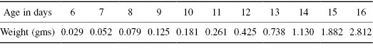
Create a scatter plot for the data in the table and overlay this with a plot of the regression line of weight with respect to age. Recall from Section 6.1 that the preferable way to analyze growth data is by using the logarithms of the exponentially increasing values. Overlay your scatter plot with a plot of the new regression line of log(weight) as a function of age. Which line (or model) appears to provide the better fit to the data?
Exercise 9.11: Obtain and plot the OLS regression of systolic blood pressure with respect to age after discarding the outlying value of 220 recorded for a 47-year-old individual.
Exercise 9.12: In a further study of systolic blood pressure as a function of age, the height and weight of each individual were recorded. The latter were converted to a Quetlet index using the formula QUI = 100*weight/height2. Fit a multivariate regression line of systolic blood pressure with respect to age and the Quetlet index using the following information:


The linear regression model is a quantitative one. When we write Y = 3 + 2X, we imply that the product 2X will be meaningful. This will be the case if X is a continuous measurement like height or weight. In many surveys, respondents use a nine-point Likert scale, where a value of “1” means they definitely disagree with a statement, and “9” means they definitely agree. Although such data are ordinal and not continuous or metric, the regression equation is still meaningful.
When one or more predictor variables are categorical, we must use a different approach. R makes it easy to accommodate categorical predictors. We first declare the categorical variable to be a factor as in Section 1.6. The regression model fit by the lm() function will include a different additive component for each level of the factor or categorical variable. Thus, we can include sex or race as predictors in a regression model.
Exercise 9.13: Using the Milazzo data of Exercise 6.20, express the fecal coliform level as a linear function of oxygen level and month. Solve for the coefficients using OLS.
Least absolute deviation regression (LAD) attempts to correct one of the major flaws of OLS, that of giving sometimes excessive weight to extreme values. The LAD method solves for those values of the coefficients in the regression equation for which the sum of the absolute deviations Σ|yi − R[xi]| is a minimum. You’ll need to install a new package in R in order to do the calculations.
The easiest way to do an installation is get connected to the Internet and then type
 install.packages("quantreg")
The installation which includes downloading, unzipping, and integrating the new routines is then done automatically. The installation needs to be done once and once only. But each time before you can use the LAD routine, you’ll need to load the supporting functions into computer memory by typing
 library(quantreg)
To perform the LAD regression, type
 rq(formula = SBP ∼ Age)
to obtain the following output:
Coefficients:
(Intercept) Age 81.157895 1.263158 To display a graph, typef = coef(rq(SBP ∼ Age))
pred = f[1] + f[2]*Age
plot (Age, SBP)
lines (Age, pred)
Exercise 9.14: Create a single graph on which both the OLS and LAD regressions for the Age and SBP are displayed.
Exercise 9.15: Repeat the previous exercise after first removing the outlying value of 220 recorded for a 47–ld individual.
Exercise 9.16: Use the LAD method using the data of Exercise 9.7 to obtain a prediction equation for systolic blood pressure as a function of age and the Quetlet index.
Exercise 9.17: The State of Washington uses an audit recovery formula in which the percentage to be recovered (the overpayment) is expressed as a linear function of the amount of the claim. The slope of this line is close to zero. Sometimes, depending on the audit sample, the slope is positive, and sometimes it is negative. Can you explain why?
The need for errors-in-variables (EIV) or Deming regression is best illustrated by the struggles of a small medical device firm to bring its product to market. Their first challenge was to convince regulators that their long-lasting device provided equivalent results to those of a less-efficient device already on the market. In other words, they needed to show that the values V recorded by their device bore a linear relation to the values W recorded by their competitor, that is, that V = a + bW + Z, where Z is a random variable with mean 0.
In contrast to the examples of regression we looked at earlier, the errors inherent in measuring W (the so-called predictor) were as large if not larger than the variation inherent in the output V of the new device.
The EIV regression method they used to demonstrate equivalence differs in two respects from that of OLS:
To compute the EIV regression coefficients, you’ll need the following R function along with an estimate of the ratio lambda of the variances of the two sets of measurements:
 eiv = function (X,Y, lambda){
 My = mean(Y)
 Mx = mean (X)
 Sxx = var(X)
 Syy = var(Y)
 Sxy = cov(X,Y)
 diff = lambda*Syy-Sxx
 root = sqrt(diff*diff+4*lambda*Sxy*Sxy)
 b = (diff+ root)/(2*lambda*Sxy)
 a = My – b*Mx
 list (a=a, b=b)
 }
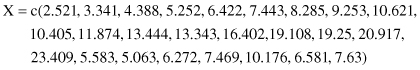
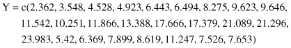
Exercise 9.18: Are these two sets of measurements comparable, that is, does the slope of the EIV regression line differ significantly from unity? Hint: Use the sample variances to estimate lambda.
Exercise 9.19: Which method should be used to regress U as a function of W in the following cases, OLS, LAD, or EIV?
To use any of the preceding linear regression methods, the following as-yet-unstated assumptions must be satisfied:
 xdiff = c(1:length(x) −1)
 ydiff = c(1:length(x) −1)
 for (i in 1:length(x)-1){
 +  xdiff[i]=  x[i+1] – x[i]
 +  ydiff[i]=  y[i+1] – y[i]
 }
Age = c(39,47,45,47,65,46,67,42,67,56,64,56,59,34,42)
SBP = c(144,220,138,145,162,142,170,124,158,154,162,
150,140,110,128)summary(lm(SBP∼Age))
A lengthy output is displayed, which includes the statements
Coefficients:
      Estimate Std.    Error       t value     Pr(>|t|)
(Intercept)  95.6125    29.8936       3.198      0.00699 **
Age           1.0474     0.5662       1.850      0.08717
This tells us that the intercept of the OLS regression is significantly different from 0 at the 1% level, but the coefficient for Age is not significant at the 5% level. The p-value 0.08717 is based on the assumption that all the random fluctuations come from a normal distribution. If they do not, then this p-value may be quite misleading as to whether or not the regression coefficient of systolic blood pressure with respect to age is significantly different from 0.
An alternate approach is to obtain a confidence interval for the coefficient by taking a series of bootstrap samples from the collection of pairs of observations (39,144), (47,220), . . . , (42,128).
Exercise 9.20: Obtain a confidence interval for the regression coefficient of systolic blood pressure with respect to age using the bias-corrected-and-accelerated bootstrap described in Section 4.2.4.
At first glance, regression seems to be a panacea for all modeling concerns. But it has a number of major limitations, just a few of which we will discuss in this section.
Whenever we use a regression equation to make predictions, we make two implicit assumptions:
We are seldom on safe grounds when we attempt to use our model outside the range of predictor values for which it was developed originally. For one thing, literally every phenomenon seems to have nonlinear behavior for very small and very large values of the predictors. Treat every predicted value outside the original data range as suspect.
In my lifetime, regression curves failed to predict a drop in the sales of ‘78 records as a result of increasing sales of 45s, a drop in the sales of 45s as a result of increasing sales of 8-track tapes, a drop in the sales of 8-track tapes as a result of increasing sales of cassettes, nor the drop in the sales of cassettes as a result of increasing sales of CDs. It is always advisable to revalidate any model that has been in use for an extended period (see Section 9.5.2).
Finally, let us not forgot that our models are based on samples, and that sampling error must always be inherent in the modeling process.
Exercise 9.21: Redo Exercise 9.7.
The exact nature of the formula connecting two variables cannot be determined by statistical methods alone. If a linear relationship exists between two variables X and Y, then a linear relationship also exists between Y and any monotone (nondecreasing or nonincreasing) function of X. Assume X can only take positive values. If we can fit Model I: Y = α + βX + ε to the data, we also can fit Model II: Y = α′ + β′log[X] + ε, and Model III: Y = α′ + β′X + γX2 + ε. It can be very difficult to determine which model if any is the “correct” one.
Five principles should guide you in choosing among models:
Exercise 9.22: Apply Model III to the blood pressure data at the beginning of Section 9.3.1. Use R to plot the residuals with the code:
 temp=lm(SBP∼Age+Age*Age)
 plot(Age,resid(temp))
What does this plot suggest about the use of Model III in this context versus the simpler model that was used originally?
Exercise 9.23: Plot the residuals for the models and data of Exercise 7.6. What do you observe?
The final two guidelines are contradictory in nature:
In order to select among models, we need to have some estimate of how successful each model will be for prediction purposes. One measure of the goodness-of-fit of the model is
where yi and  denote the ith observed value and the corresponding value obtained from the model. The smaller this sum of squares, the better the fit.
If the observations are independent, then
The first sum on the right hand side of the equation is the total sum of squares (SST). Most statistics software uses as a measure of fit R2 = 1 − SSE/SST. The closer the value of R2 is to 1, the better.
The automated entry of predictors into the regression equation using R2 runs the risk of overfitting, as R2 is guaranteed to increase with each predictor entering the model. To compensate, one may use the adjusted R2

where n is the number of observations used in fitting the model, p is the number of regression coefficients in the model, and i is an indicator variable that is 1 if the model includes an intercept, and 0 otherwise.
When you use the R function summarize(lm()), it calculates values of both R-squared (R2) and adjusted R2.
We’ve already studied several examples in which we utilized multiple predictors in order to obtain improved models. Sometimes, as noted in Section 9.4.5, dependence among the random errors (as seen from a plot of the residuals) may force us to use additional variables. This result is in line with our discussion of experimental design in Chapter 6. Either we must control each potential source of variation, measure it, or tolerate the “noise.”
But adding more variables to the model equation creates its own set of problems. Do predictors U and V influence Y in a strictly additive fashion so that we may write Y = μ + αU + βV + z or, equivalently, lm(Y ∼ U + V). What if U represents the amount of fertilizer, V the total hours of sunlight, and Y is the crop yield? If there are too many cloudy days, then adding fertilizer won’t help a bit. The effects of fertilizer and sunlight are superadditive (or synergistic). A better model would be Y = μ + αU + βV + γUV + z or lm(Y ∼ U*V).
To achieve predictive success, our observations should span the range over which we wish to make predictions. With only a single predictor, we might make just 10 observations spread across the predictor’s range. With two synergistic or antagonist predictors, we are forced to make 10 × 10 observations, with three, 10 × 10 × 10 = 1000 observations, and so forth. We can cheat, scattering our observations at random or in some optimal systematic fashion across the grid of possibilities, but there will always be a doubt as to our model’s behavior in the unexplored areas.
The vast majority of predictors are interdependent. Changes in the value of 1 will be accompanied by changes in the other. (Notice that we do not write, “Changes in the value of one will cause or result in changes in the other.” There may be yet a third, hidden variable responsible for all the changes.) What this means is that more than one set of coefficients may provide an equally good fit to our data. And more than one set of predictors!
As the following exercise illustrates, whether or not a given predictor will be found to make a statistically significant contribution to a model will depend upon what other predictors are present.
Exercise 9.24: Utilize the data from the Consumer Survey to construct a series of models as follows:
Express Purchase as a function of Fashion and Gamble
Express Purchase as a function of Fashion, Gamble, and Ozone
Express Purchase as a function of Fashion, Gamble, Ozone, and Pollution
In each instance, use the summary function along with the linear model function, as in summary(lm()), to determine the values of the coefficients, the associated p-values, and the values of multiple R2 and adjusted R2. (As noted in the preface, for your convenience, the following datasets may be downloaded from http://statcourse/Data/ConsumerSurvey.htm.)
As noted earlier, when you use the R function summary(lm()), it yields values of multiple R2 and adjusted R2. Both are measures of how satisfactory a fit the model provides to the data. The second measure adjusts for the number of terms in the model; as this exercise reveals, the greater the number of terms, the greater the difference between the two measures.
The R function step() automates the variable selection procedure. Unless you specify an alternate method, step() will start the process by including all the variables you’ve listed in the model. Then it will eliminate the least significant predictor, continuing a step at a time until all the terms that remain in the model are significant at the 5% level.
Applied to the data of Exercise 9.24, one obtains the following results:
 summary(step(lm(Purchase∼Fashion + Gamble + Ozone + Pollution)))
Start: AIC = 561.29
Purchase ∼ Fashion + Gamble + Ozone + Pollution
Df Sum of Sq RSS AIC
- Ozone 1 1.82 1588.97 559.75
- Pollution 1 2.16 1589.31 559.84
<none> 1589.15 561.29
- Fashion 1 151.99 1739.14 595.87
- Gamble 1 689.60 2276.75 703.62
Step: AIC = 559.75
Purchase ∼ Fashion + Gamble + Pollution
Df Sum of Sq RSS AIC
<none> 1588.97 559.75
- Pollution 1 17.08 1606.05 562.03
- Fashion 1 154.63 1743.60 594.90
- Gamble 1 706.18 2295.15 704.84
     summary(step(lm(Purchase∼Fashion + Gamble + Ozone + Pollution)))
Start: AIC = 561.29
 Purchase  ∼  Fashion + Gamble + Ozone + Pollution
            Df    Sum of Sq RSS        AIC
- Ozone     1    1.82          1588.97  559.75
- Pollution 1    2.16          1589.31  559.84
<none>                         1589.15  561.29
- Fashion   1    151.99        1739.14  595.87
- Gamble    1    689.60        2276.75  703.62
Step: AIC = 559.75
 Purchase ∼ Fashion + Gamble + Pollution
             Df  Sum of Sq RSS         AIC
<none>                         1588.97   559.75
- Pollution  1    17.08        1606.05   562.03
- Fashion    1    154.63       1743.60   594.90
- Gamble     1    706.18       2295.15   704.84
Call:
lm(formula = Purchase ∼ Fashion + Gamble + Pollution)
Residuals:
   Min     1Q      Median      3Q      Max
   −5.5161 −1.3955 −0.1115     1.4397  5.0325
Coefficients:
Estimate Std. Error t value Pr(>|t|) (Intercept) −1.54399 0.49825 −3.099 0.00208 ** Fashion 0.41960 0.06759 6.208 1.36e-09 *** Gamble 0.85291 0.06429 13.266 <2e-16 *** Pollution 0.14047 0.06809 2.063 0.03977 * — Signif. codes: 0***′ 0.001
From which we extract the model
E(Purchase) = −1.54 + 0.42*Fashion + 0.85*Gamble + 0.14*Pollution.
In terms of the original questionnaire, this means that the individuals most likely to purchase an automobile of this particular make and model are those who definitely agreed with the statements “Life is too short not to take some gambles,” “When I must choose, I dress for fashion, not comfort,” and “I think the government is doing too much to control pollution.”
Exercise 9.25: The marketing study also included 11 more questions, each using a nine-point Likert scale. Use the R stepwise regression function to find the best prediction model for Attitude using the answers to all 15 questions.
Linear regression techniques are designed to help us predict expected values, as in EY = μnn + βX. But what if our real interest is in predicting extreme values, if, for example, we would like to characterize the observations of Y that are likely to lie in the upper and lower tails of Y’s distribution.
Even when expected values or medians lie along a straight line, other quantiles may follow a curved path. Koenker and Hallock applied the method of quantile regression to data taken from Ernst Engel’s study in 1857 of the dependence of households’ food expenditure on household income. As Figure 9.7 reveals, not only was an increase in food expenditures observed as expected when household income was increased, but the dispersion of the expenditures increased also.
Figure 9.7 Engel data with quantile regression lines superimposed.

In estimating the τth quantile,* we try to find that value of β, for which
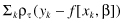
is a minimum, where
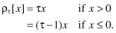
For the 50th percentile or median, we have LAD regression. In fact, we make use of the rq() function to obtain the LAD regression coefficients.
Begin by loading the Engel data, which are included in the quantreg library, and plotting the data.
 library(quantreg)
 data(engel)
 attach(engel)
 plot(x,y,xlab="household income",ylab="food
  expenditure",cex=.5)
One of the data points lies at quite a distance from the others. Let us remove it for fear it will have too strong an influence on the resulting regression lines.
 x1 = engel$x[-138]
 y1 = engel$y[-138]
Finally, we overlay the plot with the regression lines for the 10th and 90th percentiles:
plot(x1,y1,xlab="household income",ylab="food
expenditure",cex=.5)taus = c(.1,.9)
c = (max(x1)-min(x1))/100
xx = seq(min(x1),max(x1),by=c)
for(tau in taus){ + f = coef(rq((y1)∼(x1), tau=tau)) + yy = (f[1] + f[2]*(xx)) + lines(xx,yy) + }
Exercise 9.26: Plot the 10th and 90th quantile regression lines for the Engel economic data. How did removing that one data point affect the coefficients?
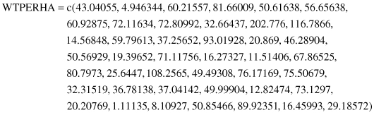
Exercise 9.27: Brian Cady has collected data relating acorn yield (WTPERHA) to the condition of the oak canopy (OAKCCSI). Plot the 25th, 50th, and 75th quantile regression lines for the following data:

As noted in the preceding sections, more than one model can provide a satisfactory fit to a given set of observations; even then, goodness of fit is no guarantee of predictive success. Before putting the models we develop to practical use, we need to validate them. There are three main approaches to validation:
In what follows, we examine each of these methods in turn.
Independent verification is appropriate and preferable whatever the objectives of your model. In geologic and economic studies, researchers often return to the original setting and take samples from points that have been bypassed on the original round. In other studies, verification of the model’s form and the choice of variables are obtained by attempting to fit the same model in a similar but distinct context.
For example, having successfully predicted an epidemic at one army base, one would then wish to see if a similar model might be applied at a second and third almost-but-not-quite identical base.
Independent verification can help discriminate among several models that appear to provide equally good fits to the data. Independent verification can be used in conjunction with either of the two other validation methods. For example, an automobile manufacturer was trying to forecast parts sales. After correcting for seasonal effects and long-term growth within each region, autoregressive integrated moving average (ARIMA) techniques were used.* A series of best-fitting ARIMA models was derived: one model for each of the nine sales regions into which the sales territory had been divided. The nine models were quite different in nature. As the regional seasonal effects and long-term growth trends had been removed, a single ARIMA model applicable to all regions, albeit with coefficients that depended on the region, was more plausible. The model selected for this purpose was the one that gave the best fit on average when applied to all regions.
Independent verification also can be obtained through the use of surrogate or proxy variables. For example, we may want to investigate past climates and test a model of the evolution of a regional or worldwide climate over time. We cannot go back directly to a period before direct measurements on temperature and rainfall were made, but we can observe the width of growth rings in long-lived trees or measure the amount of carbon dioxide in ice cores.
For validating time series, an obvious extension of the methods described in the preceding section is to hold back the most recent data points, fit the model to the balance of the data, and then attempt to “predict” the values held in reserve.
When time is not a factor, we still would want to split the sample into two parts, one for estimating the model parameters, the other for verification. The split should be made at random. The downside is that when we use only a portion of the sample, the resulting estimates are less precise.
In the following exercises, we want you to adopt a compromise proposed by C. I. Moiser.* Begin by splitting the original sample in half; choose your regression variables and coefficients independently for each of the subsamples. If the results are more or less in agreement, then combine the two samples and recalculate the coefficients with greater precision.
There are several different ways to program the division in R. Here is one way:
Suppose we have 100 triples of observations Y, P1, and P2. Using M and V to denote the values, we select for use in estimating and validating respectively,
 select = sample(100,50,replace=FALSE)
 YM = Y[select]
 P1M = P1[select]
 P2M = P2[select]
#exclude the points selected originally
 YV = Y[-select]
 P1V = P1[-select]
 P2V = P2[-select]
Exercise 9.28: Apply Moiser’s method to the Milazzo data of the previous chapter. Can total coliform levels be predicted on the basis of month, oxygen level, and temperature?
Exercise 9.29: Apply Moiser’s method to the data provided in Exercises 9.24 and 9.25 to obtain prediction equation(s) for Attitude in terms of some subset of the remaining variables.
Note: As conditions and relationships do change over time, any method of prediction should be revalidated frequently. For example, suppose we had used observations from January 2000 to January 2004 to construct our original model and held back more recent data from January to June 2004 to validate it. When we reach January 2005, we might refit the model, using the data from 1/2000 to 6/2004 to select the variables and determine the values of the coefficients, then use the data from 6/2004 to 1/2005 to validate the revised model.
Exercise 9.30: Some authorities would suggest discarding the earliest observations before refitting the model. In the present example, this would mean discarding all the data from the first half of the year 2000. Discuss the possible advantages and disadvantages of discarding these data.
Recall that the purpose of bootstrapping is to simulate the taking of repeated samples from the original population (and to save money and time by not having to repeat the entire sampling procedure from scratch). By bootstrapping, we are able to judge to a limited extent whether the models we derive will be useful for predictive purposes or whether they will fail to carry over from sample to sample. As the next exercise demonstrates, some variables may prove more reliable and consistent as predictors than others.
Exercise 9.31: Bootstrap repeatedly from the data provided in Exercises 9.24 and 9.25 and use the R step() function to select the variables to be incorporated in the model each time. Are some variables common to all the models?
In this chapter, you were introduced to two techniques for classifying and predicting outcomes: linear regression and classification and regression trees. Three methods for estimating linear regression coefficients were described along with guidelines for choosing among them. You were provided with a stepwise technique for choosing variables to be included in a regression model. The assumptions underlying the regression technique were discussed along with the resultant limitations. Overall guidelines for model development were provided.
You learned the importance of validating and revalidating your models before placing any reliance upon them. You were introduced to one of the simplest of pattern recognition methods, the classification and regression tree to be used whenever there are large numbers of potential predictors or when classification rather than quantitative prediction is your primary goal.
You were provided with R functions for the following:
You discovered that certain R functions, print() is an example, yield different results depending on the type of object to which they are applied.
You learned how to download and install library packages not part of the original R download, including library(quantreg) and library(rpart). You made use of several modeling functions including lm and rq (with their associated functions fitted, summary, resid, step, and coef), and rpart (with its associated functions prune, predict, and print). You learned two new ways to fill an R vector and to delete selected elements. And you learned how to add lines and text to existing graphs.
Exercise 9.32: Make a list of all the italicized terms in this chapter. Provide a definition for each one along with an example.
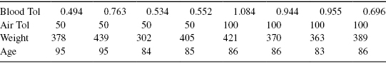
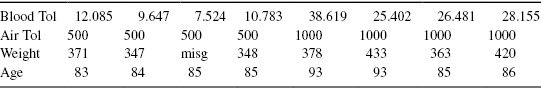
Exercise 9.33: It is almost self-evident that levels of toluene, a commonly used solvent, would be observed in the blood after working in a room where the solvent was present in the air. Do the observations recorded below also suggest that blood levels are a function of age and bodyweight? Construct a model for predicting blood levels of toluene using these data.
Exercise 9.34: Using the data from Exercise 6.18, develop a model for predicting whether an insurance agency will remain solvent.
Notes
* To ensure that the arithmetic operators have their accustomed interpretations—rather than those associated with the lm() function—it is necessary to show those functions as arguments to the I( ) function.
* τ is pronounced tau.
* For examples and discussion of ARIMA processes used to analyze data whose values change with time, see Brockwell and Davis, Time Series Theory and Methods (Springer-Verlag, 1987).
* Symposium: The need and means of cross-validation. I: Problems and design of cross-validation. Educat. Psych. Measure. 1951; 11: 5–11.
