The Black-Scholes model and Practitioner Black-Scholes model covered in Chapter 4 have the advantages that they express the option price in closed form and they are easy to implement. These models, however, make the strong assumption that the continuously compounded stock returns are normally distributed with constant mean and variance. The Black-Scholes formula does not depend on the mean of the returns, but it does depend on the volatility (the square root of the variance of returns). A number of empirical studies have pointed to time-varying volatility in asset prices and to the fact that this volatility tends to cluster. The assumption of constant volatility is the most restrictive assumption in the Black-Scholes model, so many of the advanced option pricing models encountered in the literature have sought to overcome this assumption by incorporating time-varying volatility. In this chapter we present the Heston (1993) model, a stochastic volatility model that has become popular and is relatively easy to implement in VBA.
One approach for modeling option prices under time-varying volatility is to assume that the asset price and its volatility each follow a continuous time diffusion process. Hull and White (1987) generalize the Black-Scholes model for time-varying volatility. Their model represents a general framework for stochastic volatility models in which the asset price and asset volatility each follow their own diffusion process. In their model, the option price is the expected value of the Black-Scholes price, obtained by integration over the distribution of mean volatility during the life of the option, and assuming zero correlation between the asset price and the volatility. Obtaining the density of the mean volatility requires solving a differential equation by numerical methods. While their simulations are generalized for nonzero correlation, no closed-form solution for the option price is available. Hence, while the option price expressed as the average Black-Scholes price over the mean volatility of the asset is intuitively appealing, obtaining option prices under the Hull and White (1987) model is computationally intensive.
Recall that in the model of Backus, Foresi, and Wu (2004) presented in Chapter 4, skewness and kurtosis in the distribution of the underlying asset are accounted for through a Gram-Charlier expansion of the distribution. Alternatively, incorporating skewness can be achieved by introducing correlation between the diffusion driving the underlying asset price and the diffusion driving its volatility. Incorporating skewness can be done by introducing jumps into the diffusion driving asset prices. Models with both these features are known as stochastic volatility, stochastic interest rate models with jumps (SVSI-J). Bakshi, Cao, and Chen (1997) analyze the SVSI-J model and compare its performance to the Black-Scholes model, models incorporating stochastic volatility only (SV), and models incorporating stochastic volatility and jumps (SVJ). They conclude that the most important improvement over the Black-Scholes model is achieved by introducing stochastic volatility into option pricing models. Once this is done, introducing jumps and stochastic interest rates leads to only marginal reductions in option pricing errors. Hence, in this book we ignore models that use stochastic interest rates and jumps.
Contrary to the model of Hull and White (1987), the Heston (1993) model does yield a closed-form solution. Moreover, this model is better suited at allowing correlation between the asset price and the asset volatility. The model assumes a diffusion process for the stock price that is identical to that underlying the Black-Scholes model, except that the volatility is allowed to be time varying. Hence, this model is a generalization of the Black-Scholes model for time-varying volatility. The option price is obtained by calculating the probability of a call option expiring in-the-money. Although such a probability cannot be obtained directly, it can be obtained through inversion of the characteristic function of the log price of the underlying asset.
The Heston (1993) model assumes that the stock price St follows the diffusion
where μ is a drift parameter, and z1, t is a Weiner process. The volatility  follows the diffusion

where z2, t is a Weiner process that has correlation ρ with z1, t. To simplify the implementation of the model, Ito’s lemma is applied to obtain the variance process vt, which can be written as a Cox, Ingersoll, and Ross (1985) process:
where
θ = the long-run mean of the variance
κ = a mean reversion parameter
σ = the volatility of volatility.
The time t price of a European call option with time to maturity (T − t), denoted Call(S, v, t), is given by
where
St = the spot price of the asset
K = the strike price of the option
P(t, T) = a discount factor from time t to time T
For example, assuming a constant rate of interest, r, we can write P(t, T) = e−r×(T−t). The price of a European put option at time t is obtained through put-call parity and is given by
The quantities P1 and P2 are the probabilities that the call option expires in-the-money, conditional on the log of the stock price, xt = ln[St] = x, and on the volatility vt = v, each at time t. In order to price options we need the risk-neutral dynamics, expressed here in terms of the risk-neutral parameters κ and θ.
In the appendix to this chapter it is shown how these risk-neutral versions are derived. Using these dynamics, the probabilities can be interpreted as risk-adjusted or risk-neutral probabilities. Hence,
for j = 1, 2. The probabilities Pj can be obtained by inverting the characteristic functions fj defined below. Thus,
where

In these expressions τ = T − t is the time to maturity,  is the imaginary unit, u1 = 1/2, u2 = −1/2, b1 = κ + λ − ρσ, and b2 = κ + λ. The parameter λ represents the price of volatility risk as a function of the asset price, time, volatility, and time. Although (5.2) and (5.3) are considered to be closed-form solutions, each requires evaluating the two complex integrals in (5.6). The operations on complex numbers and numerical integration procedures, defined in Chapters 1 and 2, respectively, are used to approximate these complex integrals and obtain the option prices.
 The Excel file Chapter5Heston contains the VBA code for implementing the Heston (1993) model. The file contains both the full valuation approach and the analytical closed-form approach. The valuation approach is a Monte Carlo method that requires many possible price paths to be simulated, while the analytical approach is a closed-form solution up to a complex integral that must be evaluated numerically using the methods of Chapter 2. Both of these approaches are described in the sections that follow.
This approach is a Monte Carlo simulation. A large number of stock price paths are simulated over the life of the option, using the stochastic process for St. For each stock price path, the terminal price and the value of the option at the terminal price are obtained, and the option value is discounted back to time zero at the risk-free rate. This produces the option price for a single path. This process is repeated many times, and the price of the option is taken as the mean of the option prices for each path.
Recall the Heston risk-neutral stochastic equations from (5.4):
Unfortunately, it is possible to obtain negative variances when Euler discretization is applied directly to this process. There are a number of ways to deal with this problem. The simulated variance can be inspected to check whether it is negative (v < 0). In this case, the variance can be set to zero (v = 0), or its sign can be inverted so that v becomes −v. Alternatively, the variance process can be modified in the same way as the stock process, by defining a process for natural log variances yt = ln[vt] = y, which insures a positive variance. This is the approach we use. The second equation in can easily solved for the process y = lnv by applying Ito’s Lemma:
The first equation in (5.7) and Equation (5.8) can both be discretized, which will allow the stock price paths to be simulated:
Shocks to the volatility, εv, t+1, are correlated with the shocks to the stock price process, εS, t+1. This correlation is denoted ρ, so that ρ = Corr(εv, t+1, εS, t+1) and the relationship between the shocks can be written

where εt+1 are independently and identically distributed standard normal variables that each have zero correlation with εS, t+1. Broadie and Özgür (2005) explain that the discretization in (5.9) introduces a bias in the simulation of the stock price and variance, and that a large number of time steps is required to mitigate this bias. They propose a method that simulates the stock price and variance exactly.
Using the discretized equations (5.9) it is possible to generate a stochastic volatility price path. The Excel file Chapter5Simulate contains the following VBA code to generate simulated stock paths. We illustrate this simulation using S = 100, K = 100, r = 0, τ = 180/365 = 0.5, v = 0.01, ρ = 0, κ = 2, θ = 0.01, λ = 0, and σ = 0.1. These are the same values as those used in Heston (1993).
For daycnt = 1 To daynum
e = Application.NormSInv(Rnd)
eS = Application.NormSInv(Rnd)
ev = rho * eS + Sqr(1 - rho ^ 2) * e
lnSt = lnSt + (r - 0.5 * curv) * deltat + Sqr(curv) * Sqr(deltat) * eS
curS = Exp(lnSt)
lnvt = lnvt + (kappa * (theta - curv) - lambda
* curv - 0.5 * sigmav) * deltat + sigmav
* (1 / Sqr(curv)) * Sqr(deltat) * ev
curv = Exp(lnvt)
allS(daycnt) = curS
Next daycnt
This loop generates one potential price path under the Heston stochastic volatility price process, over a time period of daynum days (daynum/365 years). Figure 5.1 shows one such possible stock price path, taken from the Excel file Chapter5Simulate. If this were the only possible price path, the option would be priced by using the terminal value of the stock price, ST = 104.26.
FIGURE 5.1 Simulated Stock Price Path

Suppose a call option with strike K = 100 is to be priced. Then the price of this call is ST − K discounted to time zero, namely (104.26 − 100)e−r×(180/365), which produces a price of $4.16 when r = 0.05. The path in Figure 5.1 is obviously not the only price path that the stock can follow, and what is needed is the distribution of the terminal stock price, which is unavailable in closed form. By simulating many stock price paths, however, this distribution can be approximated. The terminal value of the option at each simulated terminal price can be obtained, and discounted back to time zero. The option price can then be defined as the mean of the set of discounted values. The VBA function simPath(), which appears as part of the Excel file Chapter5Simulate, produces a number of simulated paths equal to the value of ITER, and evaluates the price of the call for each path.
Function simPath(kappa, theta, lambda, rho, sigmav, daynum, startS, r, startv, K)
For itcount = 1 To ITER
lnSt = Log(startS): lnvt = Log(startv)
curv = startv: curS = startS
For daycnt = 1 To daynum
' Stock Path Generating VBA Code ...
Next daycnt
Next itcount
simPath = Application.Transpose(allS)
End Function
This procedure, however, is very computationally expensive. For example, with 1,000 iterations and a call option with τ = 180 days to maturity, a total of 360,000 random standard normal variables must be generated with the NormSInv() function. In Figure 5.1 only one possible stock price path is simulated, so ITER=1.
It is straightforward to extent the code to generate the Heston (1993) call price by Monte Carlo. The Excel file Chapter5HestonMC contains the VBA function HestonMC() to perform this routine. It is the same as the function simPath(), except that the discounted call price is obtained at the end of each daycnt loop, and the function returns the average of these call prices.
Function HestonMC(kappa, theta, lambda, rho, sigmav, daynum, startS, r, startv, K, ITER)
' More VBA Code
For itcount = 1 To ITER
For daycnt = 1 To daynum
' Stock Path Generating VBA Code ...
Next daycnt
simPath = simPath + Exp((-daynum / 365) * r)*
Application.Max(allS(daynum) - K, 0)
Next itcount
HestonMC = simPath / ITER
End Function
Figure 5.2 illustrates this function on a call option with a time to maturity of 30 days. Using 5,000 iterations, the call price obtained by Monte Carlo simulation is $1.1331. The analytical price of this option, using the functions described in the latter parts of this chapter, is $1.1345.
FIGURE 5.2 Heston (1993) Call Price by Monte Carlo

The closed-form solution is much faster at producing option prices, since stock price paths do not have to be simulated. This method, however, is more difficult to implement because it requires that the complex integrals in (5.6) be evaluated. The closed-form requires the user to input the spot price St of the asset, the strike price K, the time to maturity τ = T − t, and the risk-free rate of interest r (assumed constant). It also requires estimates of the parameters driving the drift processes, namely the long-run variance θ, the current variance vt, the price of volatility risk λ, the mean reversion parameter κ, the volatility of variance σ, and the correlation between the processes driving the asset price and the volatility, ρ. Note that in earlier chapters we set t = 0 so that the time to maturity was simply T.
The Excel file Chapter5Heston contains the VBA function Heston() to implement the closed-form solution of the Heston (1993) model. This function contains four main elements:
We now describe the four different sections of the Heston() function. There are two complex integrals to be computed in (5.6), for each of the probabilities in (5.5). The VBA function HestonP1() defines the function Re[eiφln(K)f1/iφ], which is integrated to yield P1, and the function HestonP2() defines Re[eiφln(K)f2/iφ], which is integrated to yield P2.
Function HestonP1(phi, kappa, theta, lambda, rho, sigma, tau, K, S, r, v)
mu1 = 0.5
b1 = set_cNum(kappa + lambda - rho * sigma, 0)
d1 = cNumSqrt(cNumSub(cNumSq(cNumSub(set_cNum(0, rho *
sigma * phi), b1)), cNumSub(set_cNum(0, sigma ^ 2 *
2 * mu1 * phi), set_cNum(sigma ^ 2 * phi ^ 2, 0))))
g1 = cNumDiv(cNumAdd(cNumSub(b1, set_cNum(0, rho
* sigma * phi)), d1), cNumSub(cNumSub(b1,
set_cNum(0, rho * sigma * phi)), d1))
DD1_1 = cNumDiv(cNumAdd(cNumSub(b1, set_cNum(0, rho
* sigma * phi)), d1), set_cNum(sigma ^ 2, 0))
DD1_2 = cNumSub(set_cNum(1, 0), cNumExp(cNumProd(d1,
set_cNum(tau, 0))))
DD1_3 = cNumSub(set_cNum(1, 0), cNumProd(g1,
cNumExp(cNumProd(d1, set_cNum(tau, 0)))))
DD1 = cNumProd(DD1_1, cNumDiv(DD1_2, DD1_3))
CC1_1 = set_cNum(0, r * phi * tau)
CC1_2 = set_cNum((kappa * theta) / (sigma ^ 2), 0)
CC1_3 = cNumProd(cNumAdd(cNumSub(b1, set_cNum(0, rho
* sigma * phi)), d1), set_cNum(tau, 0))
CC1_4 = cNumProd(set_cNum(2, 0), cNumLn(cNumDiv
(cNumSub(set_cNum(1, 0), cNumProd(g1,
cNumExp(cNumProd(d1, set_cNum(tau, 0))))),
cNumSub(set_cNum(1, 0), g1))))
cc1 = cNumAdd(CC1_1, cNumProd(CC1_2,
cNumSub(CC1_3, CC1_4)))
f1 = cNumExp(cNumAdd(cNumAdd(cc1, cNumProd(DD1,
set_cNum(v, 0))), set_cNum(0,
phi * Application.Ln(S))))
HestonP1 = cNumReal(cNumDiv(cNumProd(cNumExp(
set_cNum(0, -phi * Application.Ln(K))), f1),
set_cNum(0, phi)))
End Function
The function HestonP2() is identical to HestonP1(), except that different values of uj and bj are used, in accordance with the definitions that follow (5.6).
Once these functions are implemented the trapezoidal integration rule from Chapter 2 can be used to obtain the integrals P1 and P2. As shown in Heston (1993), the integrals converge very quickly so a very large upper limit of integration is not needed. This will become evident later in the next section of this chapter, in which the rate of convergence of the complex integral in (5.6) is examined. In the Heston() function described below, the limits of integration are set to [0,100], and a fine grid with step size of 0.1 is used. Note that the last statements ensure that the probabilities P1 and P2 both lie in the interval [0,1].
Function Heston(PutCall As String, kappa, theta, lambda, rho, sigma, tau, K, S, r, v)
Dim P1_int(1001) As Double, P2_int(1001) As Double, phi_int(1001) As Double
Dim p1 As Double, p2 As Double, phi As Double, xg(16) As Double, wg(16) As Double
cnt = 1
For phi = 0.0001 To 100.0001 Step 0.1
phi_int(cnt) = phi
P1_int(cnt) = HestonP1(phi, kappa, theta, lambda, rho, sigma, tau,
K, S, r, v)
P2_int(cnt) = HestonP2(phi, kappa, theta, lambda, rho, sigma, tau,
K, S, r, v)
cnt = cnt + 1
Next phi
p1 = 0.5 + (1 / thePI) * TRAPnumint(phi_int, P1_int)
p2 = 0.5 + (1 / thePI) * TRAPnumint(phi_int, P2_int)
If p1 < 0 Then p1 = 0
If p1 > 1 Then p1 = 1
If p2 < 0 Then p2 = 0
If p2 > 1 Then p2 = 1
The final step of the closed-form solution is the evaluation of the call and put prices. The call price can be obtained easily by using (5.2) once the risk-neutral probabilities P1 and P2 are obtained. With the call price, put-call parity (5.3) can be used to obtain the price of the put.
HestonC = S * p1 - K * Exp(-r * tau) * p2
If PutCall = “Call” Then
Heston = HestonC
ElseIf PutCall = “Put” Then
Heston = HestonC + K * Exp(-r * tau) - S
End If
End Function
Figure 5.3 illustrates the use of the VBA functions to implement the Heston call and put prices contained in the Excel file Chapter5Heston. As in the previous chapters, range names are assigned to the 10 input values in cells C4:C13 required for the Heston() function. To obtain the price of a call, the Heston() function requires “Call” as the first argument. Hence, in cell C16 we type
FIGURE 5.3 Closed-Form Heston (1993) Option Prices


and the function produces a price of $4.0852. Similarly, to price a put option the Heston() function requires “Put” as the first argument of the function. Hence, in cell C17 we type

and the function produces a price of $1.6162.
The computational weakness of the Heston (1993) comes from the requirement of a numerical integration. The prices are sensitive to the width of the integration slices (abscissas). To increase computation speed, a Gaussian quadrature could be used, or the abscissas could be varied as a function of the φ parameter. In the next section we show how combining the functions Re[eiφ ln Kfj/iφ] leads to a function that is well-behaved and much easier to integrate.
The Heston (1993) model contains two complex integrals in (5.6), each of which are used to obtain risk-neutral probabilities. Figure 5.4 illustrates the convergence of the two functions used in (5.6). Each graph is a plot of Re[ceiφ ln Kfj/iφ] as a function of φ, j = 1, 2. Each function converges quickly to zero, and each displays a similar pattern.
FIGURE 5.4 Convergence of Functions Used in Integration
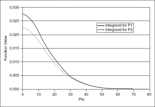
Figure 5.4 highlights two important points. First, both functions are zero for values of φ beyond, say, 75. This implies that the upper integration limits in the numerical algorithms to implement (5.6) need not be excessively high, and that the limit of 100 that we select is more than adequate. Second, the similar convergence pattern of each function implies that the integrals in (5.6) could be combined into the same integral. Recall the equation for the Heston (1993) call price (5.2)
and the expression for the risk-neutral probabilities (5.6)
These two equations can be combined to arrive at the following formula for the Heston call price:
Although this formula for the call price is less intuitive than (5.2), it combines the two sinusoidal functions into one well-behaved and fast-converging function. Figure 5.5 plots the function appearing in the integral of (5.12), as a function of φ.
FIGURE 5.5 Convergence of Combined Function

Figure 5.5 illustrates that the shape of the combined integrand in (5.12) is smooth and well behaved. Hence, using (5.12) will not cause any problems with the numerical integration required to obtain the call price. Moreover, since (5.12) requires only one numerical integration to produce the call price, rather than two integrations in (5.10), it will calculate the call price much faster. Moreover, since the integrand in (5.12) is smooth and well behaved, it will be possible to obtain accurate approximations to the integral regardless of which numerical integration algorithm is applied.
The Excel file Chapter5Integral contains the VBA function Heston2() used to generate Figures 5.4 and 5.5. The function uses the VBA functions HestonP1() and HestonP2() defined earlier in this chapter.
Function Heston2(kappa, theta, lambda, rho, sigma, tau, K, S, r, v)
Dim P1_int(1001) As Double, P2_int(1001) As Double, phi_int(1001) As Double
Dim P1 As Double, P2 As Double, phi As Double, xg(16) As Double, wg(16) As Double, HestonC As Double
Dim allP(1001, 4)
cnt = 1
For phi = 0.0001 To 100.0001 Step 0.1
phi_int(cnt) = phi
allP(cnt, 1) = phi
P1_int(cnt) = HestonP1(phi, kappa, theta, lambda, rho, sigma, tau,
K, S, r, v)
P2_int(cnt) = HestonP2(phi, kappa, theta, lambda, rho, sigma, tau,
K, S, r, v)
allP(cnt, 4) = S * P1_int(cnt) - K * Exp(-r * tau) * P2_int(cnt)
cnt = cnt + 1
Next phi
For i = 1 To 1001
allP(i, 2) = P1_int(i)
allP(i, 3) = P2_int(i)
Next i
Heston2 = allP
End Function
The output of the function is the array allP(). The values of φ are stored in the first column of allP(), while the values of the integrands for P1 and P2 are stored in the second and third columns, respectively. Finally, the value of the integrand in (5.12) is stored in the fourth column of allP().
Although regrouping both integrals into a single integral leads to greater accuracy and speed, there is another way this can be achieved. Lewis (2000) shows how the call price C(S, V, τ) for the Heston (1993) model can be written in terms of the fundamental transform Ĥ(k, V, τ), where k = kr + iki is a complex number, V is the volatility, and τ = T − t is the time to maturity. In VBA, this leads to option prices that are faster to obtain and more accurate, since only one integration is required. The general formula for the call price under a general class of stochastic volatility models is
where X = lnS/K + (r − δ)τ, ki = 1/2, and δ is the dividend yield. For Heston model, the fundamental transform takes the form
where
and where  , and c(k) = (k2 − ik)/2. When
  is set to
  . The parameter γ is the representative agent’s risk-aversion parameter (Huang and Litzenberger, 1988), and is restricted to
  . It is another way to represent the volatility risk premium. The implementation presented in Heston (1993) and shown at the beginning of this chapter, assumes risk-neutrality and specifies a form for the volatility risk premium specified by λ, where λ is restricted to be proportional to the variance. The derivation of the model presented here specifies the risk-aversion parameter of the representative agent, which implies a volatility risk premium.
The Excel file Chapter5HTrans contains VBA functions for implementing the Heston (1993) call price using the fundamental transform. The function intH() produces the integrand in (5.13). Note that in the first part of the function, the parameters κ, θ, and σ from Heston (1993) are transformed to make them consistent with the parameters ω, ξ, and θ from Lewis (2000). Hence, ω = κθ (omega), ξ = σ (ksi), and θ = κ (theta).
Function intH(K As cNum, X, V0, tau, thet, kappa, SigmaV, rho, gam) As Double
Dim b As cNum, im As cNum, thetaadj As cNum, c As cNum
Dim d As cNum, f As cNum, h As cNum, AA As cNum, BB As cNum
Dim Hval As cNum, t As cNum, a As cNum, re As cNum
omega = kappa * thet: ksi = SigmaV: theta = kappa
t = set_cNum(ksi ^ 2 * tau / 2, 0)
a = set_cNum(2 * omega / ksi ^ 2, 0)
If (gam = 1) Then
thetaadj = set_cNum(theta, 0)
Else
thetaadj = set_cNum((1 - gam) * rho * ksi
+ Sqr(theta ^ 2 - gam * (1 - gam) * ksi ^ 2), 0)
End If
im = set_cNum(0, 1)
re = set_cNum(1, 0)
b = cNumProd(set_cNum(2, 0), cNumDiv(cNumAdd(thetaadj,
cNumProd(im, cNumProd(K, set_cNum(rho * ksi, 0)))),
set_cNum(ksi ^ 2, 0)))
c = cNumDiv(cNumSub(cNumSq(K), cNumProd(im, K)),
set_cNum(ksi ^ 2, 0))
d = cNumSqrt(cNumAdd(cNumSq(b),
cNumProd(set_cNum(4, 0), c)))
f = cNumDiv(cNumAdd(b, d), set_cNum(2, 0))
h = cNumDiv(cNumAdd(b, d), cNumSub(b, d))
AA = cNumSub(cNumProd(cNumProd(f, a), t),
cNumProd(a, cNumLn(cNumDiv(cNumSub(re,
cNumProd(h, cNumExp(cNumProd(d, t)))),
cNumSub(re, h)))))
BB = cNumDiv(cNumProd(f, cNumSub(re, cNumExp(
cNumProd(d, t)))), cNumSub(re, cNumProd(h,
cNumExp(cNumProd(d, t)))))
Hval = cNumExp(cNumAdd(AA, cNumProd(BB, set_cNum(V0, 0))))
intH = cNumReal(cNumProd(cNumDiv(cNumExp(cNumProd(cNumProd(
set_cNum(-X, 0), im), K)), cNumSub(cNumSq(K),
cNumProd(im, K))), Hval))
End Function
The function HCTrans() uses the trapezoidal rule to approximate the integral in (5.13), and returns the call price. The range of integration is over (0, kmax), where  .
.
Function HCTrans(S, K, r, delta, V0, tau, ki, thet, kappa, SigmaV, rho, gam, PutCall As String)
Dim int_x() As Double, int_y() As Double
Dim pass_phi As cNum
omega = kappa * thet: ksi = SigmaV: theta = kappa
kmax = Round(Application.Max(1000, 10 / Sqr(V0 * tau)), 0)
ReDim int_x(kmax * 5) As Double, int_y(kmax * 5) As Double
X = Application.Ln(S / K) + (r - delta) * tau
cnt = 0
For phi = 0.000001 To kmax Step 0.2
cnt = cnt + 1
int_x(cnt) = phi
pass_phi = set_cNum(phi, ki)
int_y(cnt) = intH(pass_phi, X, V0, tau, thet, kappa, SigmaV, rho, gam)
Next phi
CallPrice = (S * Exp(-delta * tau) - (1 / thePI) * K *
Exp(-r * tau) * TRAPnumint(int_x, int_y))
If PutCall = “Call” Then
HCTrans = CallPrice
ElseIf PutCall = “Put” Then
HCTrans = CallPrice + K * Exp(-r * tau) - S * Exp(-delta * tau)
End If
End Function
Figure 5.6 illustrates these functions, using the same parameter values as in Figure 5.3, with ki = 0.5 and γ = 1. In cell C19 we type
FIGURE 5.6 Heston (1993) Call Price Using the Fundamental Transform


which produces a price of $4.0852, exactly that in Figure 5.3
As mentioned in the introduction to this chapter, the Heston (1993) model defines a diffusion process for the stock price that is identical to that which underlies the Black-Scholes model, except that the Heston model incorporates time-varying volatility. The volatility is allowed to be stochastic and evolves in accordance with a separate diffusion process. In this section we investigate how the incorporation of stochastic volatility affects call prices.
There are two parameters from the Heston (1993) call prices that merit particular attention, the correlation between shocks to the stock price and shocks to the variance, ρ, and the volatility of variance, σ. A negative value of ρ will induce negative skewness in the stock price distribution, so that negative shocks to the stock price will result in positive shocks to variance. This negative relationship between the stock price and variance implies that drops in the stock price are followed by increases in variance, leading to the possibility of even bigger drops in the stock price. The opposite is true when ρ is positive. How does negative or positive skewness affect option prices? When stock prices are negatively skewed, the probability of large losses is higher than predicted by the Black-Scholes model. In other words, when the correlation ρ is negative, the right tail of the stock price distribution is narrowed, and the left tail is thickened. To illustrate how this affects call prices, we replicate the experiment of Heston (1993). For different levels of moneyness, call prices are generated using the Heston model and the Black-Scholes model. For each call price, the difference between the Heston price and the Black-Scholes price is obtained, and this difference is plotted against the spot price of the stock. The same parameter values as Heston (1993) are used, namelyS = 100, K = 100, r = 0, τ = 0.5, v = 0.01, κ = 2, θ = 0.01, λ = 0, and σ = 0.225. The experiment is performed with ρ = −0.5 and repeated with ρ = +0.5, both with spot price ranging from $75 to $125 in increments of $2.50.
In order for this experiment to work properly, the volatility parameter in the Black-Scholes model must be matched to the square root of the variance parameter in the Heston model, so that the average volatility over the life of the option is the same for both models. This can be done using the characteristic functions fj defined by the model and that appear under (5.6), since moments can always be derived from the characteristic function. The volatility parameters defined in the last paragraph, however, have already been matched by Heston (1993). When rho is equal to zero (ρ = 0) the Black-Scholes volatility parameter is σBS = 0.99985, when ρ = −0.5 it is σBS = 0.099561, and when ρ = +0.5 it is σBS = 0.100409. The call prices and the differences obtained from the Heston (1993) experiments are presented in the Excel file Chapter5Correlation, and illustrated in Figure 5.7. The Heston prices are obtained using the HCTrans() function described in the previous section.
FIGURE 5.7 Impact of Correlation on Call Prices

The Black-Scholes prices use the matched volatilities that appear in cells C20 and C21. The differences between the Heston and Black-Scholes call prices appear in cells H4:H28 for ρ = −0.5 and in cells L4:L28 for ρ = +0.5. These differences are plotted as a function of the spot price in Figure 5.8.
FIGURE 5.8 Plots of Call Price Differences with Varying Correlation

The portion of Figure 5.8 to the right of the spot price of $100 corresponds to in-the-money (ITM) call options, while the portion to the left of $100 corresponds to out-of-the-money (OTM) call options. Recall that these plots are for option prices for which the underlying stock price under both models has the same average volatility over the life of the option, so the differences in call prices plotted in the figure are not due to differences in volatility. With negative correlation (dashed line) the difference for OTM options is negative, which means that OTM Heston call options are less expensive than Black-Scholes call options. Since negative correlation induces negative skewness in the stock price distribution and decreases the thickness of the right tail, the price of Heston OTM calls relative to Black-Scholes OTM calls is decreased. This result is intuitive because OTM options are sensitive to the thickness of the right tail of the stock distribution. The Heston model is able to detect this decrease in thickness and decrease the call price accordingly, whereas the Black-Scholes model is unable to detect skewness in the stock price distribution. In-the-money call options, on the other hand, are more sensitive to the left tail of the distribution. With negative correlation the left tail is thickened, so the call prices under the Heston model are higher than under the Black-Scholes model. When the correlation parameter is positive (solid line) the opposite is true. The Heston model reduces the price of ITM calls relative to Black-Scholes, but increases the price of OTM calls.
The second experiment examines the effect on call option prices of varying the volatility of variance parameter, σ. In the simplest case, a volatility of variance of zero (σ = 0), corresponds to deterministic variance in the process (5.1) driving the volatility dynamics. Volatility of variance controls the kurtosis of the return distribution. Higher volatility of variance increases the kurtosis of the distribution, while lower volatility of variance decreases the kurtosis. This experiment is identical to the previous experiment in that the difference between the call price obtained with the Heston and the call price is plotted against the spot price of the stock. The same parameters as in the previous experiment are used, but with ρ = 0. The parameter σ takes on two values, σ = 0.1 and σ = 0.2. These differences are presented in Figure 5.9, and their plots as a function of the spot price are presented in Figure 5.10. The results and the plots are in the Excel file Chapter5Variance. Again, the Heston prices are generated using the HCTrans() function described in the previous section.
FIGURE 5.9 Impact of Volatility of Variance on Call Price Differences

FIGURE 5.10 Plots of Call Price Differences with Varying Volatility of Variance

The plots in Figure 5.10 indicate that the differences between the Heston and Black-Scholes call prices are essentially symmetrical for ITM and OTM options, about the at-the-money (ATM) price of $100. The Heston model gives lower ATM call option prices than the Black-Scholes model, but higher ITM and OTM call option prices. This illustrates the fact that the volatility of variance parameter affects the kurtosis of the distribution, with little or no effect on the skewness. Higher kurtosis induces thicker tails at both ends of the returns distribution. The Heston model is able to detect these thickened tails, and increases the price of ITM and OTM calls relative to the Black-Sholes model, which cannot detect thicker tails. Not surprisingly, since higher volatility of variance induces larger kurtosis, the price difference between the Heston prices and the Black-Scholes prices is higher for σ = 0.2 than it is for σ = 0.1.
In this chapter we present the Heston (1993) option pricing model for plain-vanilla calls and puts. This model extends the Black-Scholes model by incorporating time varying stock price volatility into the option price. One simple way to implement the Heston model is through Monte Carlo simulation of the process driving the stock price. However, this method is computationally expensive. Alternatively, it is possible to obtain closed-form solutions for the option prices, but this requires that a complex integral be evaluated. Empirical experiments demonstrate that the Heston model accounts for skewness and kurtosis in stock price distributions and adjusts call prices accordingly. By combining the two integrals in the expression for the Heston (1993) call price, faster approximations to the integral are possible since only one integral must be evaluated. This is especially true when the Heston call price is obtained using the fundamental transform. The smoothness of the integrand in this combined integral suggests that good approximations to the integral are possible regardless of which numerical integration rule is used.
This section provides exercises that deal with the Heston option pricing model. Solutions to these exercises are in the Excel file Chapter5Exercises.
5.1 Use the 10-point Gauss-Legendre quadrature VBA function GLquad10() presented in Chapter 2 to implement the Heston (1993) call price, using the parameter values in Figure 5.2. Compare the results with the implementation in this chapter that uses a 1,001-point trapezoidal numerical integration.
5.2 Use the variable-point Gauss-Laguerre quadrature VBA function GLAU() presented in Chapter 2 to implement the Heston (1993) call price, using the parameter values in Figure 5.2 and varying the number of integration points (abscissas) from 1 to 16. Compare with the results implementation in this chapter that uses a 1,001-point trapezoidal numerical integration.
5.1 Instead of looping from 0.0001 to 100.0001 in the trapezoidal rule (1,001 points) the 10-point Gauss-Legendre formula requires only that the integrand be evaluated at 10 predetermined points.
Function HestonGL10(CorP, kappa, theta, lambda, rho, sigma, tau, K, S, r, v)
Dim x(5) As Double, dx As Double
Dim w(5) As Double, xr As Double, xm As Double
x(1) = 0.1488743389: x(2) = 0.4333953941
x(3) = 0.6794095682: x(4) = 0.8650633666
x(5) = 0.9739065285
w(1) = 0.2955242247: w(2) = 0.2692667193
w(3) = 0.2190863625: w(4) = 0.1494513491
w(5) = 0.0666713443
xm = 0.5 * (100): xr = 0.5 * (100)
p1 = 0: p2 = 0
For j = 1 To 5
dx = xr * x(j)
p1 = p1 + w(j) * (HestonP1(xm + dx, kappa, theta,
lambda, rho, sigma, tau, K, S, r, v)
+ HestonP1(xm - dx, kappa, theta, lambda, rho,
sigma, tau, K, S, r, v))
p2 = p2 + w(j) * (HestonP2(xm + dx, kappa, theta,
lambda, rho, sigma, tau, K, S, r, v)
+ HestonP2(xm - dx, kappa, theta, lambda, rho,
sigma, tau, K, S, r, v))
Next j
p1 = p1 * xr: p2 = p2 * xr
p1 = 0.5 + (1 / thePI) * p1
p2 = 0.5 + (1 / thePI) * p2
If p1 < 0 Then p1 = 0
If p1 > 1 Then p1 = 1
If p2 < 0 Then p2 = 0
If p2 > 1 Then p2 = 1
HestonC = S * p1 - K * Exp(-r * tau) * p2
If PutCall = “Call” Then
HestonGL10 = HestonC
ElseIf PutCall = “Put” Then
HestonGL10 = HestonC + K * Exp(-r * tau) - S
End If
End Function
The Gauss-Legendre implementation of the Heston (1993) call price is presented in Figure 5.11. The price of a call option and put option implemented with Gauss-Legendre appear in cells C19 and C20, respectively. Even with only 10 abscissas, the Gauss-Legendre method produces option prices that are identical to trapezoidal integration with 1,001 abscissas.
FIGURE 5.11 Solution to Exercise 5.1

5.2 To implement the Gauss-Laguerre quadrature, the GLAU() function is modified so that the Heston (1993) parameters can be passed to it.
Function GLAU(fname As String, n, alpha, kappa, theta, lambda, rho, sigma, tau, K, S, r, v)
' More VBA Statements
For i = 1 To n
GLAU = GLAU + w(i) * Run(fname, x(i), kappa, theta,
lambda, rho, sigma, tau, K, S, r, v)
Next i
End Function
The function HestonGLAU() calculates the Heston option price using the GLAU() function above.
Function HestonGLAU(CorP, kappa, theta, lambda, rho, sigma, tau, K, S, r, v, GLAUpoint)
Dim P1_int(1001) As Double, P2_int(1001) As Double, phi_int(1001) As Double
Dim p1 As Double, p2 As Double, phi As Double, xg(16) As Double, wg(16) As Double
Dim cnt As Integer, HestonC As Double
cnt = 1
p1 = 0.5 + (1 / thePI) * GLAU(“HestonP1”, GLAUpoint, 0,
kappa, theta, lambda, rho, sigma, tau, K, S, r, v)
p2 = 0.5 + (1 / thePI) * GLAU(“HestonP2”, GLAUpoint, 0,
kappa, theta, lambda, rho, sigma, tau, K, S, r, v)
If p1 < 0 Then p1 = 0
If p1 > 1 Then p1 = 1
If p2 < 0 Then p2 = 0
If p2 > 1 Then p2 = 1
HestonC = S * p1 - K * Exp(-r * tau) * p2
If PutCall = “Call” Then
Heston = HestonC
ElseIf PutCall = “Put” Then
Heston = HestonC + K * Exp(-r * tau) - S
End If
End Function
The Heston option price using the Gauss-Laguerre quadrature is presented in Figure 5.12. Not surprisingly, Figure 5.12 indicates that the accuracy of the option prices increases as the number of abscissas increases. With 16 points, the approximations are reasonable, but in general the approximations with Gauss-Legrendre quadratures are more accurate.
FIGURE 5.12 Solution to Exercise 5.2

In this appendix we derive the Heston (1993) risk-neutral processes for the stock price and variance. Start with the process for the stock price given by
where S = St, v = vt, and dz1 = dz1, t. By Ito’s Lemma the process for x = lnS is
The process for the square root of the variance  is
is
where β and δ are parameters, and where z2 = z2, t. Applying Ito’s Lemma, the process for the variance v is the Cox, Ingersoll, and Ross (1985) (CIR) process:
where κ = 2β, θ = δ2/(2β), and σ = 2δ. Write (5.19) as the risk-neutral process
where r is the risk-free rate, and where
The risk-neutral version of the process (5.21) for v is
where λ = λ(t, St, vt) is the price of volatility risk, and
Hence, the processes for the stock price and for the variance are
and
respectively, where
Under the probability measure P, we have z1 ∼ N(0, T) and z2 ∼ N(0, T). A new measure Q needs to be found so that  and
and  under Q. By the Girsanov Theorem, the measure Q exists provided that λ(t, St, vt) and
  satisfy Novikov’s condition. As explained in Heston (1993), Breeden’s (1979) consumption-based model applied to the CIR process yields a volatility risk premium of the form λ(t, St, vt) = λv. The process (5.27) for the variance becomes
where κ* = κ + λ and θ* = κθ/(κ + λ) are the risk-neutral parameters. In Chapter 5 we simply drop the asterisk from κ* and θ* and write the processes for the stock price and for the variance as
These are equations (5.4).