
In each table selected values are given to enable the calculation of 90%, 95%, and 99% confidence intervals using the methods described in part I. For values applicable to other levels of confidence., reference should be made to more extensive published tables such as in Geigy scientific tables.1 The first three tables can be used for calculating confidence intervals for a wide variety of statistics—such as means, proportions, regression analyses, and standardised mortality ratios—whereas the last three are for specific statistics, as described in chapter 5.
| Table 18.1 | Normal distribution |
| Table 18.2 | t distribution |
| Table 18.3 | Poisson distribution |
| Table 18.4 | Median (single sample) or differences between medians (paired samples), based on Binomial distribution with probability  |
| Table 18.5 | Differences between medians (unpaired samples), based on distributions of the Wilcoxon two sample rank sum test statistic and of the Mann–Whitney U test statistic |
| Table 18.6 | Median (single sample) or differences between medians (paired samples), based on the distribution of the Wilcoxon matched pairs signed rank sum test statistic |
The tables have been produced directly from theoretical formulae.
Table 18.1 Values from the Normal distribution for use in calculating confidence intervals
The value tabulated is z1–α/2 from the standard Normal distribution for the 100(1 – α/2) percentile and is to be used in finding 100(1 – α) % confidence intervals. For a 90% confidence interval α is 0·10, for a 95% confidence interval a is 0·05, and for a 99% confidence interval α is 0·01.

Table 18.2 Values from the t distribution for 1 to 400 degrees of freedom for use in calculating confidence intervals
The value tabulated is t1–α/2 from the t distribution for the 100(1 – α/2) percentile and is to be used in finding 100(1 – α) % confidence intervals. For a 90% confidence interval α is 0·10, for a 95% confidence interval α is 0·05, and for a 99% confidence interval α is 0·01. The relation of the degrees of freedom to sample size(s) depends on the particular application and is described in chapters 3, 4, and 8 where appropriate.
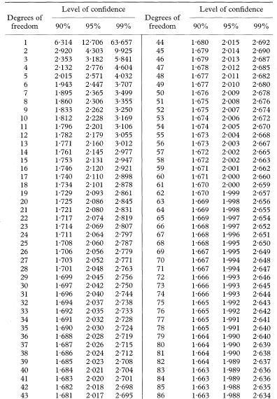
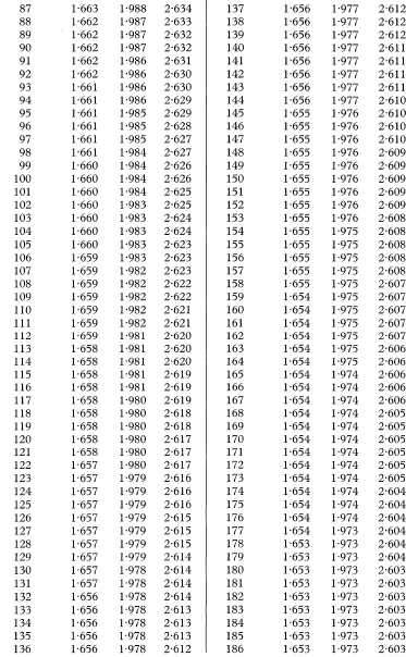
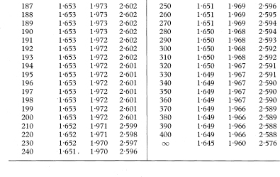
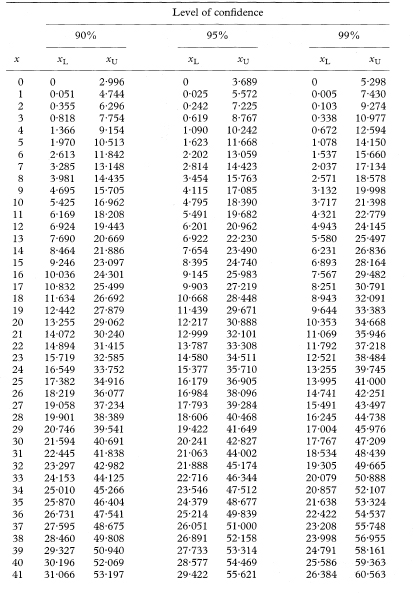
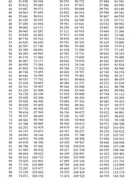
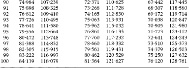
Table 18.3 Values from the Poisson distribution for observed numbers of from 0 to 100 for use in calculating confidence intervals
If x is the observed number in the study then the values tabulated (xL to xU) give the 100(1 – α)% confidence interval for the population mean, assuming that the observed number is from a Poisson distribution. For a 90% confidence interval α is 0·10, for a 95% confidence interval α is 0·05., and for a 99% confidence interval α is 0·01.
For x > 100 the following calculations can be carried out to obtain approximate values for xL and xU:

where z1–α/2 is the appropriate value from the standard Normal distribution for the 100(1 – α/2) percentile.
As an example of the closeness of the approximations to the exact values, for α = 0·05 (z1–α/2 = 1·96) and x = 100 the formulae give xL = 81·360 and xU = 121·658 for the 95% confidence interval compared to the values of xL = 81·364 and xU = 121·627 tabulated above.
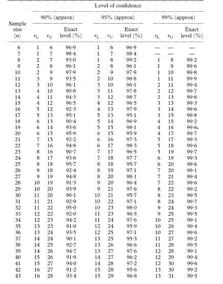
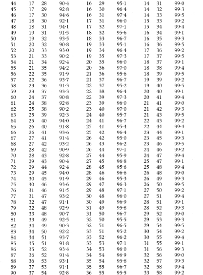
Table 18.4 Ranks of the observations for use in calculating confidence intervals for population medians in single samples or for differences between population medians for the case of two paired samples with sample sizes from 6 to 100 and the associated exact levels of confidence, based on the Binomial distribution with probability  .
.
The values tabulated (rL to rU) show the ranks of the observations to be used to give the approximate 100(1 – α)% confidence interval for the population median. For a 90% confidence interval α is 0·10, for a 95% confidence interval α is 0·05, and for a 99% confidence internal α is 0·01.
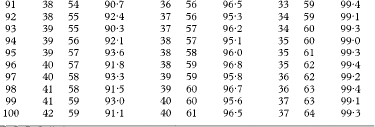
For sample sizes of n over 100, satisfactory approximations to the values of rL and rU can be found as described in chapter 5.
For n = 100 and α = 0·01, for example, the calculations give r = 37·1 and s = 63·9, which rounded to the nearest integer give rL = 37 and rU = 64 for finding the 99% confidence interval, the same values as shown in the table.
For an explanation of the use of this table see chapter 5.
Table 18.5 Values of K for use in calculating confidence intervals for differences between population medians for the case of two unpaired samples with sample sizes n1 and n2 from 5 to 25 and the associated exact levels of confidence, based on the Wilcoxon two sample rank sum distribution
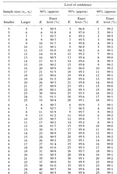
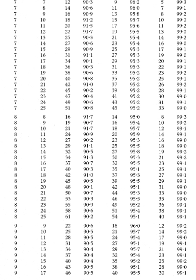
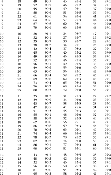
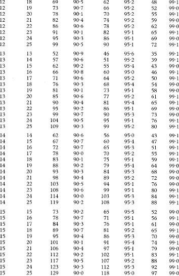
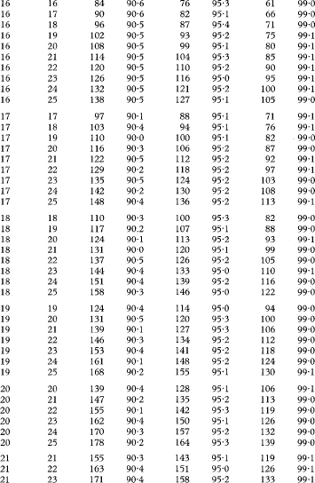
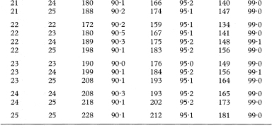
For samples sizes where n1 and n2 are greater than the range shown in the table, a satisfactory approximation to the value of K can be calculated as

rounded up to the next higher integer value, where z1–α/2 tbe appropriate value from the standard Normal distribution for the 100(1 – α/2) percentile.
For n1 = 25, n2 = 10, and α = 0·05, for example, this calculation gives 71·3, which results in K = 72 for finding the 95% confidence interval, the same value as shown in the table.
For an explanation of the use of this table see chapter 5.
Table 18.6 Values of K* for use in calculating confidence intervals for population medians in single samples or for differences between population medians for the case of two paired samples with sample size n from 6 to 50 and the associated exact levels of confidence, based on the Wilcoxon matched pairs signed rank sum distribution (see footnote overleaf)
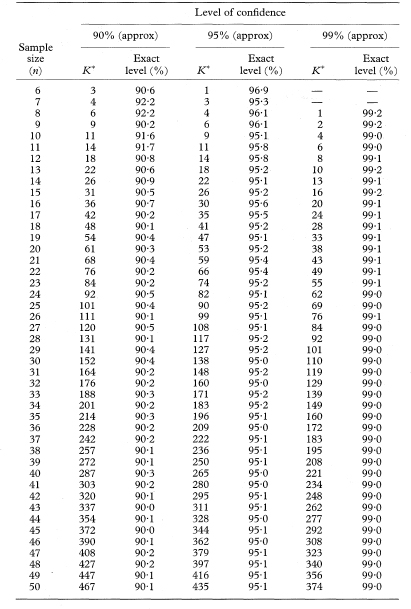
For sample sizes of n over 50, a satisfactory approximation to the value of K* can be calculated as

rounded up to the next higher integer value, where z1–α/2 is the appropriate value from the standard Normal distribution for the 100(1 – α/2) percentile.
For n = 50 and α = 0·05, for example, this calculation gives 434·5, which results in K* = 435 for finding the 95% confidence interval, the same value as shown in the table.
For an explanation of the use of this table see chapter 5.
1 Lentner C, ed. Geigy scientific tables. Vol. 2. 8th ed. Basle: Ciba-Geigy, 1982.