Comparing Research Groups: t-Test and ANOVA (F-Test)
Two types of research approaches are discussed in the literature: descriptive and inferential. Descriptive analysis is used to describe, characterize, and summarize data obtained from a selection of subjects treated as the total population. No generalizations (inferences) are made beyond the immediate N of cases. On the other hand, inferential procedures provide a set of logical methods, or rules, whereby one can make inferences with some known risk—probability—of being wrong about the conclusions to be made, concerning the larger group—population—from the findings obtained from a randomly selected sample obtained from the larger group.
When a researcher deals with the total population (no sampling), statistical inference is obviously not required, and statistical tests based on inferential rules (such as the t-test and F-test) may be inappropriate. Any observed differences between or among means are differences in the population, and inferences from sampled data to the population are unnecessary. Most research, however, rarely deals with entire populations. Generally, it is more efficient to obtain a sample, and then to make conclusions from the sample to the larger population. Thus, a systematic method (set of rules) is required for determining whether one’s findings can be generalized from the sample to the total population. Statistical inference provides this technique of generalizing with a procedure for evaluating the degree to which one might risk being wrong in their conclusions. For example, a t-test provides the basis for deciding whether the difference of means between two groups is sufficiently large to warrant generalizing a difference in the population sampled.
T-tests and F-tests (ANOVA) require appropriate measured variables to be used. For both the t-test and F-test, the X (independent) group variable must be a categorical (nominally measured) variable, and the Y (dependent) variable must be of continuous (interval or ratio) level of measurement. For example, one may wish to compare a larger group of students on two different reading methods. The large group would be divided; half the group would receive reading method A and the other half reading method B. (The reading program with the two comparison groups becomes the X independent variable (a categorical variable) in the study. After an appropriate period of time, some reading proficiency test would be given to the two groups. This reading test must yield a continuous range of scores (interval level of measurement) among the students in the two groups. This continuous variable becomes the Y dependent, or criterion variable, of the study. A mean score is computed for both groups. The two means (one for reading method A and one for reading method B) are then compared by using either a t-test or an ANOVA (F-Test). Either test is appropriate and would yield the same results for comparing only two groups. When three or more groups are compared (for example, reading methods A, B, and C), then the ANOVA F-test must be used.
Introduction: Inferential Research Methods
Again, descriptive analysis involves the description and summarization of bodies of data. If the data are from a complete enumeration of characteristics of populations (non-sample), then the summarizing measures of those characteristics (age, weight, IQ, etc.) are referred to as parameters (population parameters). Such measures include population means, modes, variances, and so on.
A major goal of science is the ability to predict behavior. Inferential methods deal with the ability to predict from a sample of data to a finite population. Thus, characteristics of populations are summarized with parameters and characteristics of samples (taken from a population) are summarized with statistics.
The ability to evaluate the degree of accuracy in summarizing from a sample to the population is also provided in the statistical tests of significance. These tests of statistical significance are incorporated in all inferential statistical procedures (t-tests, ANOVA, etc.).
Steps and Assumptions Involved in Inferential Analysis
To correctly apply inferential techniques in research, the first step is to define the population to be studied. It is important to establish the population’s boundaries and parameters, and to enumerate the number of cases and their characteristics.
The second step is to select a sample from the population. A sample is an appropriate subset of cases from the population. Inferential analysis assumes that random sampling will be employed (or some variation). Sample size must be considered also. Frequently in hypotheses testing, power analysis, or power tests, are used to determine an appropriate sample size based on the particular statistical procedure being used and the number of major research variables (independent and dependent) in the design of the study.
One of the most important steps in using inferential procedures is determining the representativeness of the sample. A nonbiased sample must be obtained in respect to all characteristics pertinent to the study. If a nonbiased sample is not obtained through simple random sampling, it may be necessary to modify the sampling frame, and perform a stratified random sample on certain key characteristics (variables). Various probability sampling techniques can be used as a means of controlling extraneous variance.
Next, one should determine the purpose for the inferential analysis. Inferential tests are used for two purposes: one for hypotheses testing and the other for estimation. Estimation involves the use of statistics, and information about the sampling distribution, to predict to a property or characteristic of the population—a population parameter.
Finally, based on the outcome of the particular statistical test, one can make generalizations, or inferences, and, in the case of estimation, predictions to the population from the sampled data.
Sampling Types and Their Characteristics
Two general categories of sampling methodologies exist. One is referred to as probability sampling and the other nonprobability. Probability samples are associated with inferential research methods. They are based on probability statistics, wherein every element in the population has an equal chance of being included in the sample. That is, they are nonbiased samples.
Nonprobability Samples
Nonprobability samples are nonrandom in nature. Bias is incurred when these sampling techniques are used. They should be avoided in inferential methods because no legitimate basis for estimating sampling error can be made. However, in other research situations, they play a legitimate role. Types of nonprobability samples are systematic samples, purposeful samples, judgment samples, quota samples, and voluntary or convenience samples.
Probability Samples
Simple random sampling means that each element (case) in the population has an equal chance of appearing in the sample. The elements of the population are listed (the order of the cases is unimportant), and a sample of cases is randomly selected to be elements of the sample. In theory, every possible combination of N elements has an equal, and independent, probability of constituting the sample. The best method of selecting a simple random sample is to use a computer-generated table of random numbers. These appear in the appendixes of most research or statistics textbooks with a brief description for their use.
Occasionally, the term sampling with replacement is used. When numbers are drawn from a hat, or some other similar method is used, then as the number is selected and recorded (corresponding to a particular subject from the population), the number should be “replaced” in the hat before another number is taken. This procedure is repeated until the total sample is drawn.
One must differentiate between random sampling and random selection. Both are based on probability sampling methods, but each has a distinct role, and unrelated purpose in research design. Random selection uses the principle of randomization to assign subjects to two or more groups in experimental designs. However, random assignment of subjects can be made, and it frequently is, without the use of sampling methodology. That is, a sample of subjects is not drawn from a population prior to conducting the random assignment process. On the other hand, one could incorporate both procedures in the design of an experimental study. If inferences, or generalizations, are to be made to a larger population from the results of the experimental study (comparison among the experimental and nonexperimental groups), then random sampling, as well as random assignment, would be necessary.
Simple stratified random sampling occurs when the population is divided into subpopulations or subsets within the larger population, and then simple random samples are taken from each subpopulation, or strata. If the subpopulations vary disproportionately in size to the total population, a better sampling design is provided if a proportionate stratified random sample is used. The size of the sample for each subpopulation is in proportion to the size of that subset in the total population. Generally, this procedure assures better representativeness of the sample in situations where a small number of cases, with important characteristics to the design of the study, are present in the total population.
Cluster sampling is used when one cannot obtain a list of all elements, or subjects, in the population necessary in conducting a random sample. In order to conduct a cluster sample, one must distinguish between primary and secondary sampling units, and clearly identify the unit of analysis for the study. For example, a research design might use teachers in a large school district as the primary sampling unit (unit of analysis). Because of the large number of teachers, it is impractical, or impossible, to obtain a complete listing of each individual. A secondary sampling unit is identified which in this example would be the schools in the district. The schools are listed, and then sampled, rather than the individual teacher. The school becomes the cluster in the sampling design. To further reduce the size of the sample (the sample obtained by clusters), teachers in each sampled school could be randomly sampled as well.
Sampling Distributions
The notion of a sampling distribution is the most important concept within inferential statistics. The sampling distribution is the distribution of possible results that could be obtained from measuring a particular statistic (for example the mean or variance) for all possible samples taken from a population. To preclude the necessity of drawing innumerable samples from a population, in order to compute these population parameters, inferential methods provide a technique of estimating these statistics from one sample.
Sampling Distribution of the Mean
The sampling distribution of the mean is defined as the probability distribution of means for all possible samples drawn from a population. For example, assume a population of 5,000 teachers from which a simple random sample of 50 teachers is selected. A mean is computed from these sampled data for a variable such as age. This procedure is repeated until 100 samples have been selected, and 100 means for the variable age have been computed. The distribution of the means of all 100 samples would constitute a sampling distribution of means. However, with inferential methods this repeated sampling is not necessary in order to estimate a population mean. One random sample is selected, and a “statistic” (the sample mean) is computed from the sample. Known information about the nature of the sampling distribution of the mean is used to generalize (infer) to the population mean (parameter).
Every statistic, whether it is a frequency, a proportion, a mean, or a variance, has a corresponding sampling distribution. There are three important properties of the sampling distribution of the mean. First, the mean of the sampling distribution equals the mean of the population. Second, the standard error of the mean equals the standard deviation of the population. And finally, the shape of the sampling distribution approximates a normal curve if the sample size is over 30.
Standard Error of the Mean
The distribution of sample means has a standard deviation referred to as the standard error of the mean. While the standard deviation measures the variability of raw scores around their mean, the standard error measures the variability of sample means around the population mean. The standard error indicates the degree of deviation of sample means about the mean of the sampling distribution. Again, this statistic is computed, or estimated, from one sample taken from the population. It indicates to what extent the estimated mean computed from the sample might be in error in generalizing to the population mean. Generally, the larger the sample size, the smaller the standard error.
Types of Inferential Approaches
Two approaches, or purposes, of inferential methods are discussed in the literature—one is hypotheses testing and the other is estimation. In order to correctly apply inferential procedures to hypotheses testing, a rather precise series of steps should be followed. Also, one should be sensitive to the distinction and importance of dealing with type I and type II errors in hypotheses testing. Establishing a level of statistical significance controls for type I error, and applying the concepts of power analysis controls for type II error.
Steps in Hypotheses Testing
Several steps are listed here which should be followed in designing research when applying inferential statistical procedures to hypotheses testing.
First, one should provide a clear and concise statement of the problem.
Second, translate the problem statement into a null hypothesis (also referred to as the statistical hypothesis), and the alternative hypothesis. The null is represented symbolically as Ho and the alternative is represented as H1. One purpose of a hypothesis test is to determine the likelihood that a particular sample could have originated from a population with the hypothesized characteristic.
Third, the specific inferential statistical test, appropriate to the research design, should be specified. Several statistical procedures are discussed in the literature that are appropriate for hypotheses testing depending on the nature of the data to be analyzed. The t-test, F-test (ANOVA), chi-square, Mann-Whitney U test, or Wilcoxon t-test are examples.
Fourth, a decision rule must be specified. This indicates when Ho will be rejected or accepted. It is based on (1) the type of statistical test being used; (2) whether a one-tailed or two-tailed test is appropriate; and (3) the level of statistical significance selected (generally, either 0.05 or 0.01). Setting the level of statistical significance will control for type I error.
Fifth, the sampling frame should be determined. This will include taking a representative random sample from the defined population, and indicating an appropriate sample size. Selecting an appropriate sample size will control for type II error.
Sixth, compute the appropriate statistic specified in step three from the sample data. If the value of the statistical test meets the level of statistical significance specified, then Ho can be rejected. If not, Ho must be accepted. That is, testing Ho can result in one of two possible outcomes:
•Accepting Ho (failing to reject) as true indicates that any trivial difference in the results (between means) are not statistically significant and, therefore, probably due to sampling error, or chance.
•Rejecting Ho as false indicates that the difference in the results (difference between means) is statistically significant and, therefore, probably due to some determining factor, or condition, other than sampling error, or chance.
•Finally, one may make generalizations and interpretations from the results of the findings. The greatest mistakes are made by many researchers at this point. What does it mean to reject or accept, Ho, and how should this be interpreted?
If one fails to reject Ho, this does not mean that the particular phenomenon, or event studied, does not exist. It only means that the study in question did not detect the event. It may exist and could be detected through replication and improvement of the research design. The failure to reject Ho is considered to be a weak decision (see earlier decision rule), because little, or no, generalization can be made from the lack of findings in the data. When Ho is rejected, then this is considered to be a strong decision, because one can report a definitive conclusion as to the results of the study.
Type I and Type II Error
A well conceptualized hypothesis test must be concerned with both the probability of a type I error (alpha) in the event that Ho is true, and a type II error (beta) in the event that Ho is false.
The probability of a type I error is controlled by establishing the level of statistical significance. The probability of a type II error is controlled by establishing the level of the sample size (B beta). To reduce B, the likelihood of a type II error, one should increase the sample size. Prior to beginning a study, a power analysis can be conducted by consulting the appropriate tables for the particular statistical test to identify the sample size that guarantees a hypothesis test that will control for both type I and type II error. In addition to sample size, effect size and level of statistical significance must be determined (see the following discussion of power analysis).
Committing a type I error (alpha) is to reject the Ho when it is true. Ho is true but rejected; that is, a false alarm. A type I error is to conclude falsely that a difference exists in the data when in fact it does not, or the difference is only trivial. For example, if one were comparing the difference between means from two groups (a t-test), and concluded that the difference was significant and meaningful when in fact the difference was trivial and slight (or due to sampling error, chance, or too large of a sample size), a type I error has been committed. This happens frequently in research in education where tests of statistical significance are used inappropriately—especially, when a sample size is used which is too large for the particular statistical test.
A type I error occurs when, just by chance, a sample mean strays into the rejection region for the true Ho. If a researcher is concerned about the possibility of type I error, or wishes to control more carefully for this likelihood, it can be established by setting the level of statistical significance from 0.05 to 0.01, or lower (0.001). Setting the level of statistical significance is also referred to as alpha.
Type II error (beta) is to retain (not reject) Ho when it is false. Ho is false but not rejected; that is, a miss. A type II error is committed when one concludes, falsely, that a difference does not exist, when in fact a difference does exist, but was not detected due to a small effect size, a small sample size, and/or the particular statistical test employed. For example, if one were comparing the difference between means from two groups (a t-test), and concluded due to the modest, or small, effect size (small difference between the two means) that this difference was trivial, and not statistically significant, when in fact the difference did represent a meaningful difference in the population, then a type II error has been committed. This can occur when the sample size is too small for the particular statistical test. Much research in the social sciences is misinterpreted when tests of statistical significance are computed with inappropriate sample sizes for the particular statistical test employed. Thus, this stresses the importance of conducting a power analysis to determine correct sample size before the research is started (Cohen, 1969).
When there is a large effect size, or a seriously false Ho (when a large difference between means exist), a type II error is less likely to occur. A type II error is more likely to occur when Ho is mildly false, or when a moderate effect size (small difference between means) is present.
If it is important to reject a small, or moderately false, Ho (small or moderate effect size), then the probability of type II error can be reduced by increasing the sample size (N of cases). Again, to obtain the correct balance between controlling for the probability of type I or type II error, one should conduct a power analysis for the particular statistical test employed.
Power Analysis
The power of a statistical test from a nontechnical perspective is the ability of that test to detect a false null hypothesis (Ho). The probability that the test will lead to the rejection of the null hypothesis. Power is the probability that the test will yield statistically significant results. That it will result in the conclusion that the phenomenon under study exists.
The power (beta) of a statistical test depends on establishing values for three parameters. These are the significance criterion (alpha), sample size, and the effect size (ES).
•The significance criterion (alpha) is a value that represents the standard of “proof” that the phenomenon exists, by determining whether a one-tail or two-tail test is appropriate. This is accomplished by setting the level of statistical significance. Typically, statistical convention dictates a significance level of either 0.05 or 0.01, even though there is no mathematical or statistical theory to support this.
•Sample size is a value which establishes the reliability or precision of a sample once taken from the population. It is the closeness with which the sample value can be expected to approximate the relevant population value. The larger the sample size, other things being equal, the smaller the error, and the greater the reliability, or precision, of the results (the ability of the statistical test to detect a difference, or an effect).
•Effect size is the degree to which the phenomenon under study indeed is present (Ho is false), or absent (Ho is true). The null hypothesis always means that the effect size is zero (no difference between means). The effect size is some specific nonzero value in the population. Effect size serves as an index of the degree of departure from the null hypothesis.
With these three values—significance level, sample size, and effect size—one can determine the power of the particular statistical test to detect the phenomenon under study by using power tables established for each statistical test. This constitutes a post hoc analysis. In addition to a post hoc analysis, one can also determine an appropriate sample size (N or cases) prior to conducting a study by establishing three elements: level of significance (alpha), estimated effect size (ES), and power.
Thus, a minimum sample size required for any given statistical test can be determined as a function of ES, alpha, and power. The researcher estimates the anticipated effect size, sets a level of statistical significance, and specifies the power desired. Then the minimum sample size (N of cases) for the particular statistic can be determined. This approach to power analysis should be employed in the design of all hypotheses testing studies in order to determine the correct sample size (Cohen, 1969).
For example, a researcher who is using the Pearson correlation decides to have a power equal to 0.80 (suggesting a 20 percent chance of violating a type II error) in order to detect a population correlation coefficient of r = 0.40 (the effect size) at the 0.05 level of significance (five chances in 100 of violating a type I error). The minimum sample size (N of cases) for this statistical analysis would require 46 subjects (Cohen, 1969). More advanced statistical texts will provide tables and methods of computing the sample size based on a power analysis.
As an example, Cohen (1969) provides information for conducting a power analysis for the t-test statistic. The notation at the top of the table—a1 = 0.05—indicates that this table is to be used in testing a hypothesis with a one-tail test (directional hypothesis) at the 0.05 level of statistical significance. Corresponding tables exist in various combinations for testing other possibilities—a2, two-tail tests (nondirectional hypotheses), and 0.01 level of statistical significance. Again, by setting effect size (r value, column headings at the top of the table) and power desired (numbers within the table), the sample size (N of cases) can be determined—the column on the far left under the heading n.
For example, a median effect size of r = 0.40 and a power of 0.80 would indicate a minimum sample size of 37 subjects. As the t-test requires two groups (two means are compared), each group would require 37 subjects. If the estimate of the effect size can be increased to r = 0.50 with a power of 0.80, then the sample size can be reduced to only 23 subjects for each group. Or, if one wished to increase power to 0.90, then the sample size would be 30 subjects. By studying the table, one can conduct a number of different scenarios for selecting sample size and for better understanding the close relationship among effect size, sample size, power, and statistical significance in correctly testing hypotheses.
Several sources are available for conducting power tests as either post hoc analyses, or more importantly, prior to commencing a study. Several are provided in the references at the end of this book.
Establishing correct sample size, balanced for the potential of violating either type I or type II error, is fundamental to good research design, but often neglected or misunderstood by many researchers. A sample size too large may be as serious as a sample size that is too small. A point that must be remembered is that finding, or failing to find, a significant result is often more a function of sample size than the intrinsic truth, or falsity, of the null hypothesis. Given the four components discussed earlier, it is clear that a major aspect of the power of a test is the size of the sample. Power increases as the sample size increases. For a large sample, almost any deviation from the null hypothesis—any value greater than zero—will result in a statistically significant result.
Thus, sample size either too large, or too small, can cause serious problems. An excessively large sample (N of cases) translates into an extra sensitive test that may detect even a very small effect that lacks practical importance. A too small sample translates into an insensitive test that misses even a relatively large, important effect.
The importance of this is that an essentially arbitrary factor—the sample size—can often determine the conclusion reached in a test of statistical significance, if it is mechanically applied and misinterpreted. This can be further aggravated by significance tests themselves, since the choice of a level of significance is not based on any mathematical, statistical, or substantive theory. The choice is totally arbitrary, based on convention or tradition. In much research, the absurdity of adhering rigidly to arbitrary significance levels has to be apparent to the competent researcher, as it substitutes a mechanical procedure for mature, scientific, and sensible judgment.
Estimation
Estimation involves the use of a statistic based on sample data, and knowledge about the sampling distribution, to predict or infer to a property, or characteristic, of the population—a population parameter. For example, one can compute the mean from sample data, and then estimate the population mean (µ) for the characteristic within some limits of error—the confidence interval.
The confidence interval specifies a range of values, above and below the estimated mean, which includes the unknown population mean for a certain percent of the time (generally either 95 percent or 99 percent). A higher confidence level of 99 percent produces a wider, less precise, estimate. Also, the larger the sample size, the smaller the standard error, and thus, a more precise (narrower) confidence interval.
There is a close relationship between the standard error and the confidence interval. Remember, the standard deviation of the sampling distribution is the standard error. The standard error is a measure of sampling error, and it is used to determine the range of values for the confidence interval. If the standard error is known, then one can calculate the probability of being far from the mean of the distribution. For example, in a normal distribution approximately 68 percent of the cases fall within one standard deviation (standard error) of the mean. Thus, the standard error provides a range about the mean in which 68 percent of the samples taken from the population should include the population mean. Or, 68 percent of the time, the estimated mean should fall within the range of the standard error about the mean.
Assume that a mean for the variable age is computed from sample data, and the value 46 years is obtained. A standard error of 3.7 years is also computed. It could be concluded that 68 percent of the time (or if we took more samples, 68 percent of the samples) the estimated mean would fall between 42.3 years and 49.7 years. In this example, the confidence level is set at 68 percent, or at one standard error above and below the mean.
Confidence intervals can be set at whatever level one desires. Generally, either 95 percent or 99 percent levels are used. With normally distributed data, the 95 percent confidence interval extends 1.96 standard errors above and below the sample statistic (in this example, the mean). A 99 percent confidence interval extends 2.575 standard errors above and below the sample statistic. Of course the 99 percent confidence interval is a wider, less precise, range of values than the 95 percent confidence interval.
Analysis of Variance—ANOVA (F-Test)
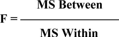
The basic concern of the ANOVA statistical model is to determine the extent to which group means differ, and to determine if the difference between, or among, group means is statistically significant—not just due to sampling error or a chance occurrence. The principle involved in ANOVA is to compare the variability among group means (called MS between) with the average variability of scores within each group about the group’s mean (called MS within). If the variability between, or among, group means is large in comparison to the within group variability of scores around the individual group means, then it can be concluded that the group means probably come from different populations, and that there is a statistically significant difference. The statistical test that provides this solution is referred to as the F-Ratio or F-Test. The basic formula is:
Unfortunately, ANOVA is a misleading name. Analysis of Means would be more appropriate inasmuch as it deals with whether the means of a variable differ from one group of observations to another. It employs ratios of variances (variability of scores about the mean within groups compared to variability of means between or among groups) in order to determine if the difference in the value of the means are statistically significant. The major assumptions that apply to ANOVA, as a parametric procedure, are:
•The observations, or scores, within each group must be mutually independent (as opposed to a repeated measures ANOVA).
•The variances (standard deviations) within each group must be approximately equal—homogeneity of variances.
•The variations within each group should be from normally distributed populations.
•The contributions to variance in the total sample must be additive. ANOVA is an additive model. Each score can be decomposed into three sources of variance:
∘Each score contributes to the overall mean, or mean of means, across all groups.
∘Deviation of each group mean from the overall mean.
∘Deviation of each individual score (within group deviation) from the group mean.
There are several types of ANOVA designs discussed in the literature. For example, one-way ANOVA, N-way ANOVA, Fixed and Random Effects models, and Repeated Measures designs are only a few. Each type is characterized by the number of independent variables included in the design, the sampling technique, or the use of the N of cases. Table 3.1 distinguishes some of the characteristics among basic types of ANOVA designs.
Table 3.1. Types of Basic ANOVA Designs
|
One-way ANOVA |
Two-way or n-Way ANOVA |
|
|
Fixed |
One Independent Var. |
Two or more Independent Variables |
|
Effects |
Single Classification |
(e.g., 2X2, 2X3 Factorial Designs) |
|
Model |
All categories of IV must be included |
Two or more Main Effects and Interaction Effects |
|
Random |
One Independent Var. |
Two or more Independent Variables |
|
Effects |
Single Classification |
|
|
Model |
Only a sample of categories of the Independent Variable used |
|
|
Other types of ANOVA models: Repeated Measures Design Three or more Independent Variable Designs (Factorials) Latin Squares or Counter Balanced Designs Nested Designs Regression Models |
||
Each of the ANOVA designs closely parallel, or accompanies, a particular experimental research design. Most often the two are synonymous. A Repeated Measures ANOVA is a Repeated Measures research design. A study of most ANOVA designs cannot be treated separately from experimental methodology. Similarly, experimental research methodology should not be discussed separately from a consideration of various ANOVA models.
ANOVA Example
The one-way ANOVA example (table 3.2) will be helpful in visualizing, and better understanding, the computations employed in the analysis.
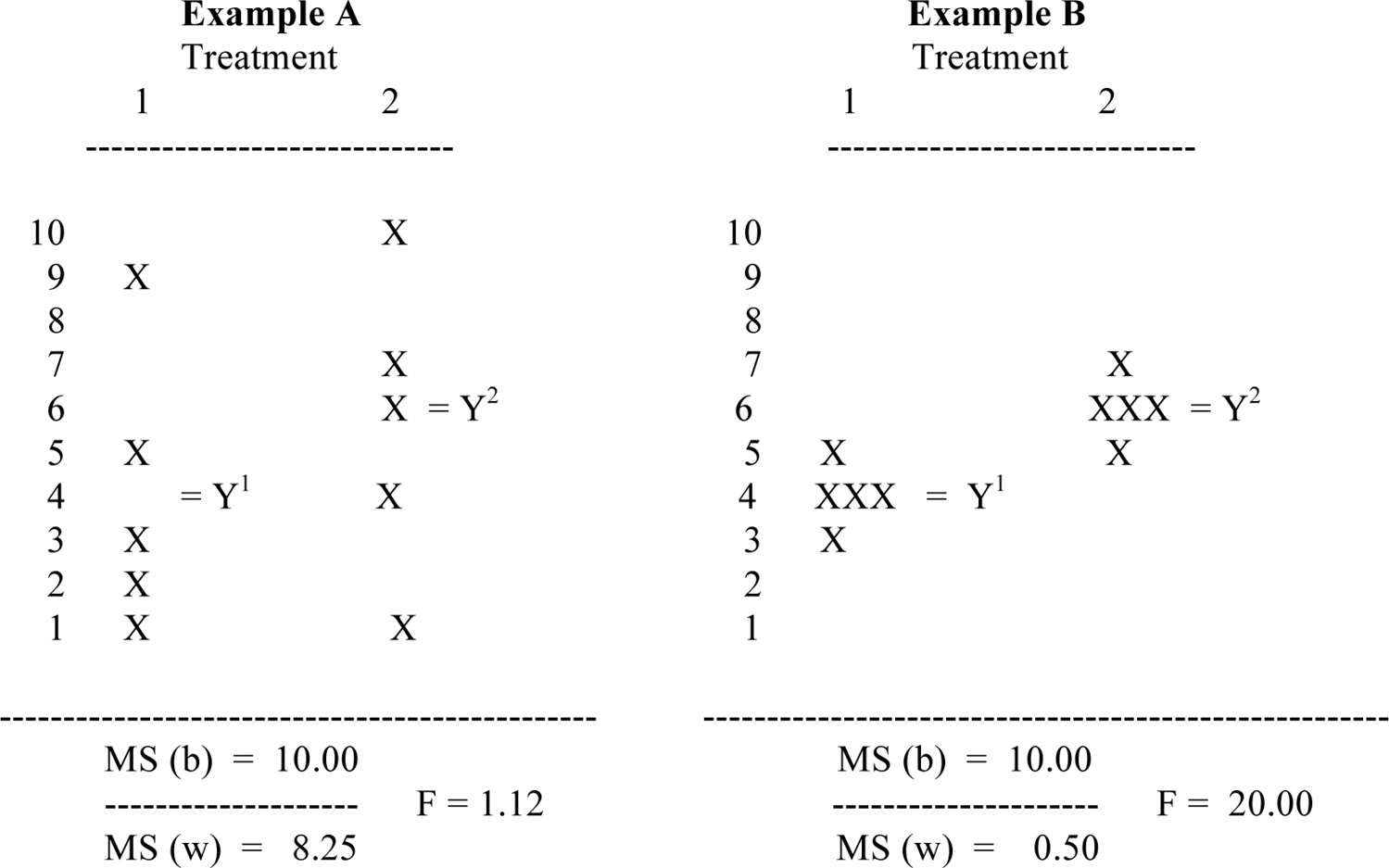
Table 3.2. ANOVA Example
In both examples A and B, the difference between the means (Y1 and Y2) is identical, Y1 = 4 and Y2 = 6. The MS between groups is 10.00. In example A, the within group variation is spread out from the mean yielding a large computation of MS within (8.25), and thus a very small F ratio (F = 1.15). In contrast in example B, the within group variation around the mean is much smaller—closer to the mean—and the computation of MS is negligible (0.50). Thus, the F ratio (F = 20.00) between group variation divided by within group variation for example B is a large value and, therefore, statistically significant.
The within group variance (MS) is also referred to as the error term, or as the residual. Obviously, the greater the spread of scores around the mean within the each group, the greater the error in the model, and the least likely is statistical significance to be achieved.
t-Test and ANOVA—Analysis and Interpretation: Example Computer Statistical Program
The data used in the following computer examples are the same data introduced in chapter 1 (Table 1.6), with the five X, independent variables, and BSTRESS (burnout and stress) as the Y, dependent variable. In addition, the research (teacher survey) determined other ancillary (moderating) variables, such as teachers’ age, grade level taught (elementary, middle school, or high school), years of teaching, and gender. The variables grade level with three categories and gender with two categories are appropriate categorical (nominal) variables to be used in a t-test or ANOVA (F-test) analysis.
T-test and one-way ANOVA (bivariate) are similar inferential tests. T-tests are used primarily for hypotheses testing of the difference of means between two groups (e.g., gender—male, female) or among two or more groups for ANOVA (school level with three categories—elementary, middle school, and high school). Thus, in order to properly use these tests, one needs a categorical (group) X variable and an interval measured Y variable—a continuously scored variable where a mean can be appropriately computed.
Both the t-test and ANOVA are generally associated with experimental or quasi-experimental research methods. The t-test answers the question: Is the difference between two sample means (the Y variable) statistically significant? Typically, one mean represents an experimental group receiving some treatment, and the other mean represents a control or comparison group (no treatment condition). However, one may compare three, or more, treatments simultaneously, such as four different teaching methods. This then requires ANOVA. It answers the question: Is the variability among groups large enough in comparison with the variability within groups to justify the inference that the means of the populations from which the different groups were sampled are not the same? If the mean of the treatment group is significantly different from the nontreatment group, then one can conclude that some experimental effect (referred to as the “main effect”) due to the treatment occurred.
When comparing means from only two groups, the results from the t-test and the F-test are identical. The only difference is an arithmetic one. That is, the F-value is always the square of the t-value for the same variables and data. For example, compare the F-test for the variables gender and age with the t-test results. The F ratio (2.47) is approximately the square of the t-value (1.581) for the same data. ANOVA must be used when the independent, X, variable has three or more categories. In the ANOVA example, school level is used with three categories—elementary, middle school, and high school.
t-test
In the following examples, the t-test is performed with gender (dichotomous variable) as the X, independent variable and age, decision making, income, job satisfaction, SBP, teacher authority, years of teaching, and role ambiguity as the various Y, dependent variables. Thus, in any analysis several dependent variables may be tested simultaneously.
In addition to using t-tests and F-tests for experimental or quasi-experimental research, they may be used also for descriptive purposes. In these examples, one is simply interested in determining a difference between males and females, from the research sample, on personal variables such as age and income, and scores on other major research variables.
For each t-test procedure, three separate tables are produced—a Group Statistics table, Levene’s Test for Equality of Variances table, and the Independent Samples Test (t-test) table. Different computer statistical programs may produce slightly different tables, or may omit some tables. However, the Independent Samples Test is the main t-test table, providing the t-value and test of statistical significance for each variable in the analysis.
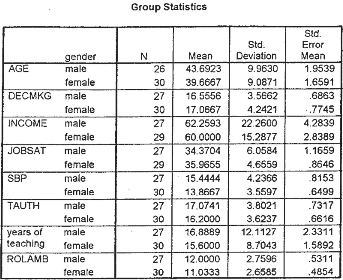
The Group Statistics table provides basic statistics for each dependent variable used in the analysis. For example for the variable age, there are 26 males and 30 females, mean score for age for the males is 43.69 and for the females 39.67, and the standard deviation for each group is provided.
The Equality of Variances (Table 3.3) provides a test for the homogeneity of variance. Both t-tests and F-tests require that the group variances (standard deviations) be equal, or near equal (homogeneous), between the two groups. (Recall, the variance and standard deviation are essentially the same thing. The only difference is one of arithmetic, where the variance is the square of the standard deviation. For analysis and interpretation purposes, standard deviation is used because it corresponds numerically to the mean.) For example, the standard deviations between male and female on age are 9.9630 and 9.0871, indicating that the two variances (standard deviations) are nearly equal (homogeneous). The statistical test to determine homogeneity of variance is provided with the F-value in the first column of Levene’s Test for Equality of Variances table.
If the F-value is statistically significant (Sig) P = 0.05 or smaller, this indicates that the variances of the two groups (that is, the standard deviations) are not equal. For example, the F-test for income is F = 6.418, (Sig) P = 0.014, which is much smaller than P = 0.05 and, therefore, statistically significant. Thus, the t-value obtained from the “Equal variances not assumed” must be used (Independent Samples t-test table). On the other hand, if the F-test is not statistically significant (P = 0.051 or larger), this indicates that the variances for the two groups (standard deviations) are equal, or nearly equal; therefore, the t-value for the “Equal variances assumed” should be used. For example, the F-value for age is F = 0.034, nearly zero, and the “Sig” test is P = 0.854. Thus, the Equal Variances Assumed t-value (t = 1.581) should be used.
In the Equality of Variances table, the variables of Income and Years of Teaching both have large F-values with Sig values less than P = 0.05 (0.014 and 0.013, respectively), indicating statistical significance. Thus, the “Equal variances not assumed” t-tests (t = 0.440 for Income and t = 0.457 for Years of Teaching) should be used for the t-test from the Independent Samples Test table.
Again, the t-test provided in the Independent Samples Test table provides the individual t-test for each variable in the analysis. In the third column of this table, a two-tailed test of statistical significance is provided for each t-value. For example, the t-test for the variable AGE indicates that there is not sufficient difference between the two group means, males = 43.7 and females = 39.7 (t = 1.581), to obtain a statistically significant result. In fact, there is no statistical significance for any of the comparisons between the variables analyzed in this example.


One-Way ANOVA, F-test
As indicated previously, when comparing means from three or more groups, the F-test must be used. However, the F-test provides only a gross overall test of statistical significance among group means. It does not indicate among which pairs of group means that statistical significance exists. If only one pair of means are statistically significant—regardless of how many combinations of pairs can be formed (with a four category variable six possible pairs exist)—the F-test will be significant. Thus, when one obtains a significant F ratio, a post hoc analysis (multiple comparisons test) must be performed to determine which pair, or pairs, of group means are statistically significant. These tests are provided in most comprehensive statistical programs. Several post hoc tests exist—such as Scheffe, Duncan—however, the Scheffe test provides the most conservative estimate of statistical significance.
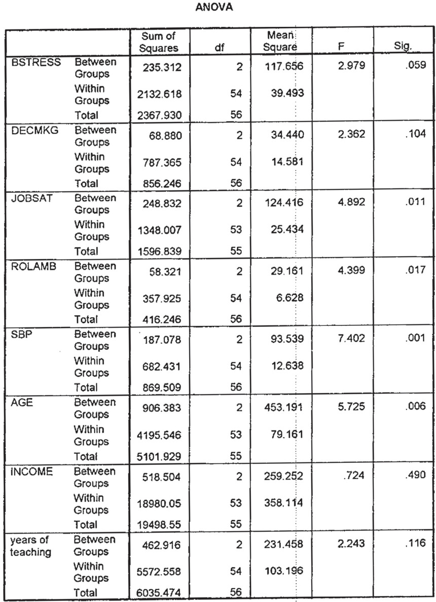
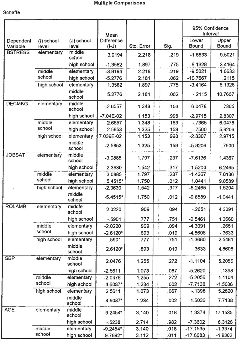
For the variables in the following example (see the ANOVA data in Table 3.4), the Y variables of Jobsat, Rolamb, SBP, and Age have F-ratios sufficiently large to indicate a statistical significant result (Sig column has a value smaller than P = 0.05). Inasmuch as the X variable, school level in this analysis, has three categories (elementary, middle school, and high school), it is not clear among which possible pairs that the test of statistical significance has occurred. That is, the possible comparisons (pairs) are elementary with middle school, elementary with high school, and middle school with high school. Again, the F-test provides only an overall indication that at least one of the possible comparisons (pairs) are statistically significant. It does not indicate which comparison. In order to determine this, a Multiple Comparisons must be conducted. As indicated earlier, several tests are available in most statistical programs; however, the Scheffe test is the most conservative and frequently used. The table marked “Multiple Comparisons” below provides the analysis to determine which group means are statistically significant at the P = 0.05 level.
For the variable Jobsat, the only test of statistical significance smaller than P = 0.05 (sig column) is for the comparison (pair) between the high school and middle school categories. The difference between the two means is −5.4515 and statistical significance (P = 0.012). The negative mean difference score of −5.4515 between high school and middle school indicates that the mean score was higher for the high school. That is, high school teachers indicated a higher level of job satisfaction than middle school teachers. For the variable Age, statistical significance exists between elementary and middle school (P = 0.018) and middle school and high school (P = 0.011), but not between elementary school and high school (P = 0.982). For SBP (student behavioral problems, i.e., student discipline problems), the significant difference (P = 0.002) is between the middle school and high school teachers’ responses. Again, the negative mean difference score between middle schools and high schools suggests that the middle school teachers indicated more problems with students discipline than the high school teachers.