Exercise 18.1.

Find the values of λ2 for which the boundary value problem
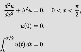
has nontrivial solutions.
These midterm examinations are actual exams held during the academic term, and each lasted 50 minutes.
Exercise 18.1.
Find the values of λ2 for which the boundary value problem
has nontrivial solutions.
Solution.
Case (i): λ = 0. In this case, the general solution to d2u/dx2 = 0 is given by u(x) = Ax + B, and u(0) = 0 implies that B = 0, so that u(x) = Ax. The condition  implies that
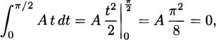
which implies that A = 0, and the boundary value problem has only the trivial solution in this case.
Case (ii): λ ≠ 0. In this case, the general solution to d2u/dx2 + λ2u = 0 is given by

and u(0) = 0 implies that A = 0 so that u(x) = B sin λx. Now , implies that
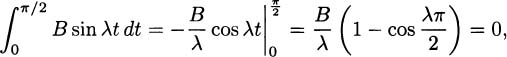
so either B = 0 or cos(λπ/2) = 1. Therefore, a nontrivial solution exists if and only if we have cos(λπ/2) = 1; that is, λπ/2 = 2πn, where n ≠ 0 is an integer. The values of λ2 for which the boundary value problem has nontrivial solutions are

for n = 1, 2, 3, ….
Exercise 18.2.
Let f(x) = cos2 x, 0 ≤ x ≤ π, and f(x + 2π) = f(x) otherwise.

Solution.
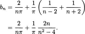
 bn sin nx, the coefficients bn in the Fourier sine series are computed as follows:


Exercise 18.3.
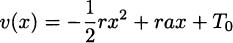
Let v(x) be the steady-state solution to the boundary value-initial value problem
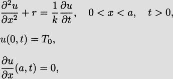
where r is a constant. Find and solve the boundary value problem for the steady-state solution v(x).
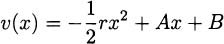
Solution. The steady-state solution v(x) satisfies the boundary value problem

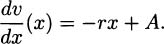
and the general solution to the differential equation is
and
Therefore,

while
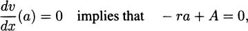
so that

The steady-state solution is therefore
for 0 ≤ x ≤ a.
Exercise 18.4.
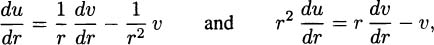
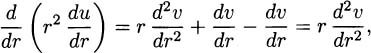
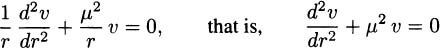
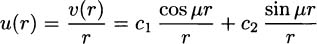
The neutron flux u in a sphere of uranium obeys the differential equation
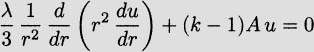


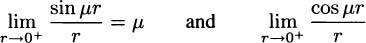
Solution.


Exercise 18.5.

Show that

 , find the Fourier cosine series of the function f(x) = sin x, for 0 ≤ x ≤ π, and then use Dirichlet’s theorem.
Solution. For 0 ≤ x ≤ π, the Fourier cosine series is

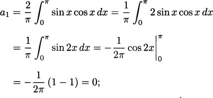
For n = 0,

for n = 1,
and for n > 1,

The Fourier cosine series for sin x on the interval 0 ≤ x ≤ n is therefore

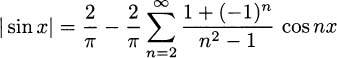
Since cos nx is an even function, this is also the Fourier series for the even extension of sin x, that is, | sin x|, on the interval –π ≤ x ≤ π, so that

and since this is a continuous piecewise smooth function on –π ≤ x ≤ π such that | sin(–π)| = |sin π| = 0, then by Dirichlet’s theorem the Fourier series converges to |sin x| for all x ∈[–π, π], and
for all x ∈ [–π, π]. However, |sin x| is a continuous periodic function on the interval –∞ < x < ∞, so the Fourier series converges to | sin x| for all x, – ∞ < x < ∞.
Exercise 18.6.
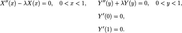
Solve Laplace’s equation in the square 0 < x, y < π with the boundary conditions

Solution. We use separation of variables and assume a solution to Laplace’s equation

of the form u(x, y) = X(x) · Y(y). Separating variables, we have
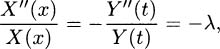
and we obtain the two ordinary differential equations
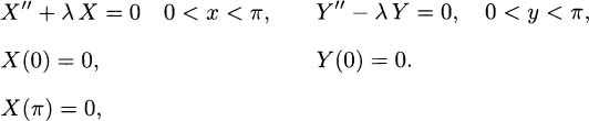
Solving the complete boundary value problem for X, the eigenvalues and eigenfunctions are given by

for n > 1. The corresponding problem for Y is

with solutions
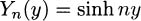
for n ≥ 1.
From the superposition principle, we write

and setting y = π, we need

and from the orthogonality of the eigenfunctions,

so that
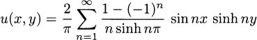
for 0 < x < π, 0 < y < π.
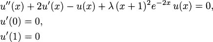
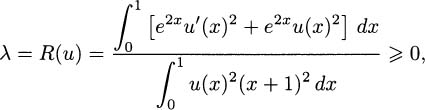
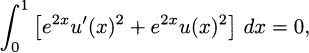
Exercise 18.7.
Consider the following eigenvalue problem on the interval (0,1):

Solution.


Exercise 18.8.
Consider Laplace’s equation for the steady-state temperature distribution in a square plate of side length 1.

Obviously, the solution is u(x, y) = 1 for 0 ≤ x ≤ 1, 0 ≤ y ≤ 1. Show that this is the case by using separation of variables.
Solution.
Using separation of variables, assume that u(x,y) = X(x) · Y(y), and obtain the two boundary value problems
Note that we cannot meet the boundary conditions u(0,y) = u(l,y) = 1 for all 0 < y < 1 by requiring that X(0) = 1 and X(l) = 1.
We solve the complete boundary value problem for Y first since it has homogeneous boundary conditions. The eigenvalues are λn = n2π2 and the corresponding eigenfunctions are
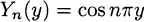
for n = 0,1,2, The corresponding solutions to the problem for X are

for n ≥ 1.
From the superposition principle, we have

for 0 < x < 1 and 0 < y < 1. Applying the boundary condition u(0,y) = 1, we get
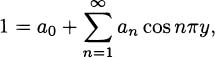
and from the orthogonality of the eigenfunctions on the interval [0,1], this implies that

The solution is now

for 0 < x < 1 and 0 < y < 1. Applying the boundary condition u(l, y) = 1, we get

that is,
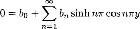
for 0 < y < 1. Again, from the orthogonality of the eigenfunctions on the interval [0,1], this implies that

Therefore, the solution is u(x, y) = 1 for 0 ≤ x ≤ 1, 0 ≤ y ≤ 1, as promised.
Exercise 18.9.

Solve the normalized wave equation

Solution. Since the partial differential equation and the boundary conditions are linear and homogeneous, we can use separation of variables, and assuming a solution of the form u(x, t) = ϕ(x) · G(t), we get two ordinary differential equations:

where λ is the separation constant. We solve the spatial problem first since it has a complete set of boundary conditions. These are homogeneous Dirichlet conditions, so the eigenvalues and eigenfunctions are given by

for n ≥ 1, and the corresponding solutions to the temporal equation are

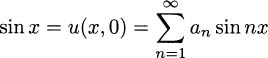
Using the superposition principle, we write the solution as an “infinite” linear combination of {ϕn · Gn}n≥1; that is,

where the constants an and bn are determined from the initial conditions
and
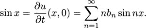
From the orthogonality of the eigenfunctions, we find

and the solution is

for 0 < x < π, and t > 0.

Solution. Following the hint, the differential equation becomes

with general solution

for 0 < x < 1. Applying the first boundary condition, we have

so that

Applying the second boundary condition, we have

so that

and we have a nontrivial solution if and only if
for some μ ≠ 0. However, the graphs of y = tanhμ and y = hμ intersect only at μ = 0 if h ≥ 1, and they intersect at exactly one positive value μ0 if 0 < h < 1. Therefore, there is exactly one negative eigenvalue for this Sturm-Liouville problem if and only if 0 < h < 1, and the eigenvalue is

where μ0 is the positive root of the equation tanhμ = hμ. The corresponding eigenfunction is
for 0 ≤ x ≤ 1.
Exercise 18.11.
Consider Laplace’s equation


Solve this problem using separation of variables.
Solution. Assuming a solution of the form u(r,0) = R(r) · φ(0), and separating variables, we have the following problems for R and φ:

We solve the θ-problem first. The eigenvalues and corresponding eigenfunctions are

for n ≥ 1. The corresponding r-equation is the Cauchy-Euler equation

with general solution

for n ≥ 1. The boundedness condition |R(0)| < ∞ requires that Bn = 0, so that

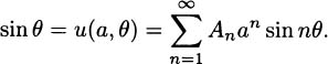
for n ≥ 1. Using the superposition principle, we write

for 0 r a, 0 < θ < λ, and from the boundary condition we want
From the orthogonality of the eigenfunctions on the interval [0,π], we have

so the solution is

for 0 < r < a, 0 < θ < π λ.